Validation: discrepancy assessment

A general measure of validation assessment is demonstrated herein to characterise the discrepancy between the quantitative predictions from a model, and relevant empirical data when predictions and data may both contain aleatory and epistemic uncertainty. This measure has a specific focus on imprecise probability.

This extends beyond the deterministic world when the predicted quantity is a scalar (real) value. In fact, we recognise the case when predictions or data contain epistemic uncertainty that cannot be well characterised with any single probability distribution.

In this tutorial, we will explore the different cases of uncertainty representation in either the prediction or observation.

from pyuncertainnumber import pba, area_metric
import matplotlib.pyplot as plt

plt.rcParams.update({
        "font.size": 11,
        "text.usetex": True,
        "font.family": "serif",
        "figure.figsize": (6, 4.5),
        "legend.fontsize": 'small',
        })

def verify_area_metric(a, b, ax=None):
    am = area_metric(a, b)

    if ax is None:
        fig, ax = plt.subplots()
    a.plot(ax=ax, fill_color='salmon', bound_colors=['salmon', 'salmon'], label='a', nuance='curve')
    b.plot(ax=ax, label='b', nuance='curve')
    ax.set_title(f"area metric: {am:.5f}")
    plt.show()

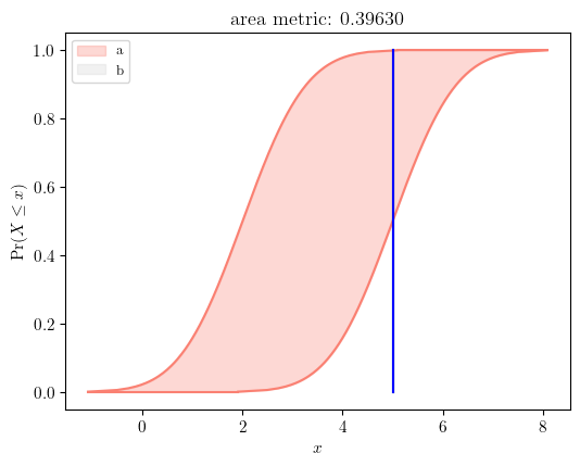
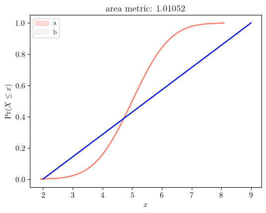
Example case 1: two distributions

a = pba.normal(5, 1)
b = pba.uniform(2, 9)
verify_area_metric(a, b)

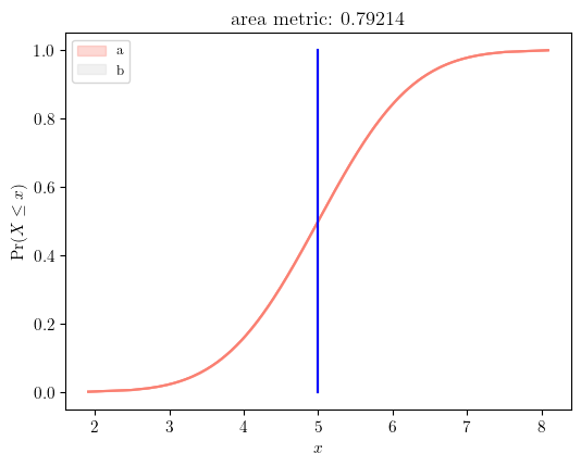
Example case 2: a distribution and a scalar value

NUMBER = 5.0
a = pba.normal(5, 1)
b = pba.I(NUMBER).to_pbox()
verify_area_metric(a, b)

Example case 3: p-boxes that overlap

a = pba.normal([2, 5], 1)
b = pba.uniform([2, 4], [7,9])
verify_area_metric(a, b)

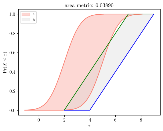
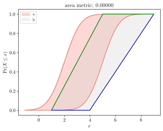
Example case 4: p-boxes that have imposition

a = pba.normal([2, 5], 1)
b = pba.uniform([1, 4], [5,9])
verify_area_metric(a, b)

Example case 5: a p-box and a scalar value

a = pba.normal([2, 5], 1)
b = pba.I(5).to_pbox()
verify_area_metric(a, b)