pyuncertainnumber.calibration
Submodules
- pyuncertainnumber.calibration.calibration
- pyuncertainnumber.calibration.data_peeling
- pyuncertainnumber.calibration.epistemic_filter
- pyuncertainnumber.calibration.iterative_filtering
- pyuncertainnumber.calibration.knn
- pyuncertainnumber.calibration.mcmc
- pyuncertainnumber.calibration.pdfs
- pyuncertainnumber.calibration.tmcmc
- pyuncertainnumber.calibration.utils_bayesian
Classes
Class for TMCMC implementation |
|
Container for one TMCMC stage. |
|
Calibration via Bayesian MCMC (e.g. Metropolis-Hastings, HMC, NUTS). |
|
Unified kNN-based calibrator for black-box models or precomputed simulations. |
|
The EpistemicFilter method to reduce the epistemic uncertainty space based on discrepancy scores. |
Package Contents
- class pyuncertainnumber.calibration.TMCMC(N: int = None, parameters: list = None, names: list[str] = None, log_likelihood: callable = None, mutation_steps: int = 5, status_file_name: str = None, trace=None)
Class for TMCMC implementation
- Parameters:
N (int) – number of particles to be sampled from posterior
parameters (list) – list of (size Nop) prior distributions instances
log_likelihood (callable) – log likelihood function on \(\theta\) to be defined which is problem specific
status_file_name (str) – name of the status file to store status of the tmcmc sampling
- Returns:
- returns trace file of all samples of all tmcmc stages.
At stage m: it contains [Sm, Lm, Wm_n, ESS, beta, Smcap]
- Return type:
mytrace
Example
>>> from pyuncertainnumber.calibration.tmcmc import TMCMC
>>> from pyuncertainnumber import pba
>>> # create an instance of TMCMC class and run tmcmc
>>> parameters = [pba.D("uniform", (0.8, 2.2)), pba.D("uniform", (0.4, 1.2))] # dummy prior distributions
>>> t = TMCMC(
>>>     N=1000,                                             # number of particles
>>>     parameters=parameters,                              # prior distributions
>>>     names =['k1', 'k2'],                                # parameter names
>>>     log_likelihood=log_likelihood_function,             # user defined log likelihood function
>>>     mutation_steps=1,                                   # number of MCMC steps for perturbation
>>>     status_file_name='tmcmc_progressing_status.txt',    # status log file
>>> )
>>> mytrace = t.run()
>>> # for loading trace file
>>> import pickle
>>> with open('tmcmc_trace.pkl', 'rb') as f:
>>>     mytrace = pickle.load(f)
>>> re = TMCMC(trace=mytrace, names=names)                  # create TMCMC instance with loaded trace and names
>>> re.plot_updated_distribution(save=False)                # plot prior and posterior distribution
>>> prior_samples = re.load_prior_samples()                 # load prior samples as DataFrame
>>> posterior_samples = re.load_posterior_samples()         # load posterior samples as DataFrame
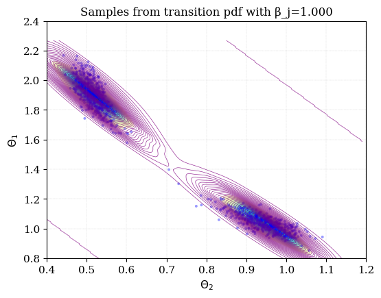
Example of TMCMC calibration of a 2-DOF system
- N = None
- parameters = None
- names = None
- log_likelihood = None
- mutation_steps = 5
- status_file_name = None
- trace = None
- check_names()
- run() list[Stage]
Run the TMCMC algorithm
- Returns:
returns trace file of all samples of all tmcmc stages.
- Return type:
mytrace
- check_trace()
- save_trace(mytrace, file_name: str, save_dir=None)
Save the trace to a file
- Parameters:
mytrace – trace file of all samples of all tmcmc stages.
file_name (str) – name of the file to save the trace
- load_prior_samples(trace=None) pandas.DataFrame
- load_posterior_samples(trace=None) pandas.DataFrame
- plot_updated_distribution(trace=None, save=False)
Plot the prior and posterior distribution of the parameters
- Parameters:
trace – trace file of all samples of all tmcmc stages.
save (bool) – if True, save the figure
- class pyuncertainnumber.calibration.Stage
Container for one TMCMC stage.
- Parameters:
Sm (NDArray) – samples before resampling (N x Np)
Lm (NDArray) – log-likelihoods at Sm (N,)
Wm_n (NDArray) – normalized incremental weights (N,)
ESS (Optional[float]) – effective sample size the next stage (can be None in terminal stage)
beta (float) – tempering parameter next stage beta
Smcap (Optional[NDArray]) – resampled samples (N x Np), None in terminal stage
- Sm: numpy.typing.NDArray
- Lm: numpy.typing.NDArray
- Wm_n: numpy.typing.NDArray
- ESS: float | None
- beta: float
- Smcap: numpy.typing.NDArray | None
- __repr__() str
- property samples: numpy.typing.NDArray
Samples before resampling (from previous stage).
- property log_likelihoods: numpy.typing.NDArray
Log-likelihood evaluated at samples.
- property weights: numpy.typing.NDArray
Normalized incremental importance weights.
- property effective_sample_size: float | None
Effective sample size after reweighting the next stage.
- property tempering_parameter: float
Tempering parameter beta next stage beta.
- property resampled_samples: numpy.typing.NDArray | None
Samples after importance resampling (before MH mutation).
- class pyuncertainnumber.calibration.MCMCCalibrator(n_chains: int = 4, n_samples: int = 1000, burn_in: int = 200)
Bases:
CalibratorCalibration via Bayesian MCMC (e.g. Metropolis-Hastings, HMC, NUTS).
- n_chains = 4
- n_samples = 1000
- burn_in = 200
- _prior = None
- _likelihood = None
- _posterior_chain = None
- setup(prior=None, likelihood=None, model=None)
Define priors and likelihood (or simulator-based likelihood).
- calibrate(observations: Any, resample_n: int | None = None) Any
Run MCMC to sample posterior given observations.
- get_posterior() Any
Return MCMC chain or posterior samples.
- class pyuncertainnumber.calibration.KNNCalibrator(knn: int = 100, a_tol: float = 0.05, evaluate_model: bool = False)
Bases:
CalibratorUnified kNN-based calibrator for black-box models or precomputed simulations.
- Parameters:
knn (int) – Number of neighbors per observed row. Default: 100.
a_tol (float) – Tolerance for matching simulated \(\xi\) to a requested \(\xi^*\) (when reusing). A simulation is kept if \(\|\xi_{\text{sim}} - \xi^*\|_\infty < a_{\text{tol}}\). Default: 0.05.
evaluate_model (bool) – If True, call the black-box model for each \(\xi\) in
xi_liston a shared \(\theta\) grid. If False, reusesimulated_data(requires y/theta/xi arrays). Default: False.random_state (int) – Seed for reproducibility (affects theta_sampler and resampling). Default: 42.
Note
Setup (unified approach):
If
evaluate_model=Falseandsimulated_datais provided:Reuse pre-computed simulations
Build a per-design kNN index by filtering rows with \(\|\xi - \xi^*\|_\infty < a_{\text{tol}}\) for each \(\xi^*\) in
xi_list
If
evaluate_model=True:Simulate \(y = \text{model}(\theta, \xi)\) for each \(\xi\) in
xi_listUse a shared \(\theta\) grid drawn once from
theta_sampler(n_samples)Build per-design kNN indices on this shared grid
Calibration workflow (single/multi-design):
For each observation pair \((y_{\text{obs}}, \xi)\):
Standardize \(y_{\text{obs}}\) using the per-design scaler
Find k nearest neighbors in y-space
Map neighbor indices to \(\theta\) values for that design
Stack \(\theta\) samples across all observations/designs (or apply voting/intersection)
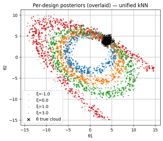
KNN calibration illustration.
- knn = 100
- a_tol
- evaluate_model = False
- random_state = 42
- _theta_grid: numpy.ndarray | None = None
- _theta_by_xi: Dict[Tuple[float, Ellipsis], numpy.ndarray]
- _y_by_xi: Dict[Tuple[float, Ellipsis], numpy.ndarray]
- _scaler_by_xi: Dict[Tuple[float, Ellipsis], sklearn.preprocessing.StandardScaler]
- _neigh_by_xi: Dict[Tuple[float, Ellipsis], sklearn.neighbors.NearestNeighbors]
- _grid_idx_by_xi: Dict[Tuple[float, Ellipsis], numpy.ndarray]
- _posterior: Dict[str, Any] | None = None
- _sim_y: numpy.ndarray | None = None
- _sim_theta: numpy.ndarray | None = None
- _sim_xi: numpy.ndarray | None = None
- static _key_from_xi(xi) Tuple[float, Ellipsis]
Stable tuple key for a scalar/vector design ξ.
- setup(model: Callable[[numpy.ndarray, float | numpy.ndarray], numpy.ndarray] | None = None, theta_sampler: Callable[[int], numpy.ndarray] | None = None, simulated_data: Dict[str, numpy.ndarray] | None = None, xi_list: List[float | numpy.ndarray] | None = None, n_samples: int = 10000)
Prepare per-design kNN structures by either reusing simulated_data or simulating for each design.
- Parameters:
model (callable, optional) – Black-box simulator with signature
model(theta, xi) -> y(vectorized over theta).theta_sampler (callable, optional) – Sampler for \(\theta\); required when
evaluate_model=True.simulated_data (dict, optional) – Dict with keys {“y”: (n, dy), “theta”: (n, dθ), “xi”: (n, dξ)} when reusing sims.
xi_list (list, optional) – List of designs; each item can be scalar or array-like. If None, defaults to [0.0].
n_samples (int) – Number of \(\theta\) samples to draw when
evaluate_model=True. Default: 10000.
- nearest(y: numpy.ndarray | List[float], xi: float | numpy.ndarray, k: int | None = None, return_dist: bool = False)
Return k nearest neighbors for y at design xi.
- Parameters:
y (array-like) – Query outputs, shape (m, d_y) or (d_y,).
xi (scalar or array-like) – Design key to select the per-design index.
k (int, optional) – Number of neighbors; defaults to
self.knn.return_dist (bool) – If True, also return distances and raw indices. Default: False.
- Returns:
Shape (m*k, dθ) stacked \(\theta\) for all query rows. distances (ndarray, optional): Returned if
return_dist=True. indices (ndarray, optional): Returned ifreturn_dist=True.- Return type:
theta_neighbors (ndarray)
- calibrate(observations, resample_n: int | None = None, combine: str = 'stack', combine_params: dict | None = None)
Run kNN calibration and aggregate posterior θ across neighbor-hit blocks.
- Parameters:
observations – Observed simulator or model outputs to calibrate against.
resample_n (int | None) – If set, resample posterior θ samples to this size. If None, return all aggregated θ without resampling.
combine (str) –
Aggregation mode. One of:
’stack’: concatenate all kNN θ; optional de-duplication.
’intersect’: retain θ hit at least min_count times across neighbor blocks.
combine_params (dict | None) –
Optional parameters controlling aggregation and KDE weighting.
Supported keys:
dedup (bool): Default False. Remove duplicate θ (only for ‘stack’).
theta_match_tol (float): Default 1e-9. Tolerance or rounding quantum for comparing/merging θ values.
min_count (int | None): Minimum occurrences for ‘intersect’. Default is max(1, ceil(0.5 * total_blocks)), meaning θ must appear in about half of neighbor lists.
use_kde (bool): Default False. If True, fit KDE on aggregated θ to compute log-scores and normalized weights.
kde_bandwidth (float | None): Bandwidth for KDE. If None (default), use Scott’s rule.
Tip
Two aggregation modes are supported:
stack: Concatenate all kNN θ into a single array. Supports optional de-duplication of nearly identical θ values.
intersect: Keep θ values that occur in at least min_count neighbor blocks across all observations/design points (default ≈ half of all blocks).
Optional density weighting via KDE can be applied after aggregation to compute normalized posterior weights.
- Returns:
- A dictionary with keys:
’mode’ (str): Always ‘knn’.
’theta’ (ndarray): Posterior samples of shape (N, dθ); resampled if resample_n is provided.
’weights’ (ndarray | None): None for stack/intersect, or a length-N array of KDE weights if use_kde=True.
’meta’ (dict): Aggregation info; may include KDE bandwidth if density weighting is used.
- Return type:
dict
- _round_rows(A: numpy.ndarray, tol: float) tuple[numpy.ndarray, numpy.ndarray]
Round rows of A to multiples of tol and return (unique_rows, counts).
- Parameters:
A (ndarray) – Input array to process.
tol (float) – Tolerance for rounding. If tol <= 0, exact matching is used.
- Returns:
- (unique_rows, counts) where unique_rows are the deduplicated rows
and counts are the occurrence counts.
- Return type:
tuple
- _kde_logweights(X, bw=0.5, n_max_exact=5000)
Compute KDE-based log-weights for posterior samples X.
- Parameters:
X (ndarray) – Posterior samples, shape (n, d).
bw (float) – Bandwidth for Gaussian kernel. Default: 0.5.
n_max_exact (int) – Max n for exact pairwise KDE. Above this, fall back to sklearn.KernelDensity. Default: 5000.
- Returns:
logp (ndarray): Log-density values at X, shape (n,).
w (ndarray): Normalized weights, shape (n,).
- Return type:
tuple
- get_posterior() Any
Return the last computed posterior dict; raises if calibrate() hasn’t been called.
- class pyuncertainnumber.calibration.EpistemicFilter(xe_samples: numpy.typing.NDArray, discrepancy_scores: numpy.typing.NDArray = None, sets_of_discrepancy: list = None)
The EpistemicFilter method to reduce the epistemic uncertainty space based on discrepancy scores.
- Parameters:
xe_samples (NDArray) – Proposed Samples of epistemic parameters, shape (ne, n_dimensions). Typically samples from a bounded set of some epistemic parameters.
discrepancy_scores (NDArray, optional) – Discrepancy scores between the model simulations and the observation. Associated with each xe sample, shape (ne,). Defaults to None.
sets_of_discrepancy (list, optional) – List of sets of discrepancy scores for multiple datasets. Each element should be an NDArray of shape (ne,). Defaults to None.
Tip
For performance functions that output multiple responses, some aggregation of discrepancy scores may be used. Depending on the number of observation, either a single set of discrepancy scores or multiple sets can be provided.

Convex hull with bounds illustration.
- xe_samples
- discrepancy_scores = None
- sets_of_discrepancy
- filter(threshold: float | list)
Filter the epistemic samples based on a discrepancy threshold.
- Parameters:
threshold (float | list) – The discrepancy threshold(s) for filtering data points.
- Returns:
the filtered xe samples;
hull;
lower bounds;
upper bounds of the bounding box, or (None, None) if unsuccessful.
- Return type:
tuple
- iterative_filter(thresholds: list) list
Iteratively filter the epistemic samples based on multiple thresholds.
- Parameters:
thresholds (list) – List of discrepancy thresholds for filtering data points.
simulation_model (callable, optional) – A function that takes xe_samples as input and returns discrepancy scores. Required if re_sample is True. Defaults to None.
Note
thresholds are assumed to be sorted in ascending order.
- iterative_filter_w_simulation_model(thresholds: list, re_sample: bool = False, simulation_model=None)
Iteratively filter the epistemic samples based on multiple thresholds.
- Parameters:
thresholds (list) – List of discrepancy thresholds for filtering data points.
re_sample (bool, optional) – If True, re-evaluate discrepancy scores at each iteration using the simulation_model. Defaults to False.
simulation_model (callable, optional) – A function that takes xe_samples as input and returns discrepancy scores. Required if re_sample is True. Defaults to None.
Note
if re_sample is True, the simulation_model should be provided to re-evaluate discrepancy scores.
- filter_on_sets(plot_hulls: bool = True)
Filter the epistemic samples based on multiple sets of discrepancy scores.
- Parameters:
plot_hulls (bool, optional) – If True, plots the convex hulls of the first five sets. Defaults to True.
- Returns:
lower bounds;
upper bounds of the intersected bounding box, or (None, None) if unsuccessful
- Return type:
tuple
Note
self.sets_of_discrepancy must exist.
- plot_hull_with_bounds(filtered_xe, hull=None, ax=None, show=True, x_title=None, y_title=None, hull_alpha=0.25)
Plot the convex hull and bounding box of the epistemic samples.
- Parameters:
hull (ConvexHull, optional) – Precomputed convex hull. If None, it is computed.
ax (matplotlib Axes, optional) – Existing axes to draw on. If None, a new figure/axes is created.
show (bool, optional) – If True, calls plt.show() at the end. Defaults to True.
x_title (str, optional) – Label for the x-axis. Defaults to None.
y_title (str, optional) – Label for the y-axis. Defaults to None.
hull_alpha (float, optional) – Transparency of the hull surface. Defaults to 0.25.
- Returns:
The axes containing the plot.
- Return type:
ax (matplotlib Axes)