Transitional MCMC with the classic eigenvalue problem
TMCMC (Transitional Markov Chain Monte Carlo) has been widely used in stochastic model updating, which aims to find the posterior samples of the parameters (\(\theta\)) to be updated given empirical observations.
This notebook provides a hands-on example that illustrates how TMCMC is used in a classic eigenvalue problem with only elementary knowledge about structural dynamics.
Consider a simple two-degree-of-freedom system under undamped free vibrations. The equation of motion reads:
Assuming harmonic response yields the classic eigenvalue problem:
this further leads to the characteristic equation by a nontrivial solution using the determinant:
where
eigenvalues: a system of 2 degrees of freedom will give a polynomial of 2th degree in \(\lambda\). The 2 roots will represent the frequencies at which the undamped system can oscillate in the absence of external forces, i.e., natural frequencies of the system.
eigenvectors: The values of the vector \(\phi\) at each natural frequency describe the mode shape of the corresponding mode of vibration, which reflects the relative displacement pattern between the two masses.
This setup solves the natural frequencies given known stiffness and mass matrix. Inversely, in order to identify the system given empirical measurements, consider a problem of solving the stiffness of the system given a few measurements of the \(\lambda_1\) which is contaminated by some Gaussian noise (e.g. known standard deviation \(\sigma_{\lambda_{1}}\)).
Note
To further explore the identifiability of the system, Yuen (2010) proposes 3 different setups:
Given one measured eigenvalue
Given two measured eigenvalues
Given a set of eigenvalue and associated eigenvector (mode shape)
Readers are encouraged to have a think on the other two problems.
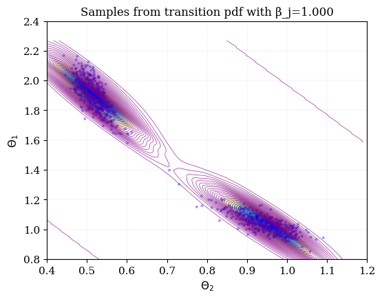
This notebook provides an exemplar solution for the problem 2 where noisy data on two eigenvalues are available to infer the stiffness parameters. Ground truth values are \(\theta_{1} = \theta_{2} = 1.0\), and priors are assumed as \(\theta_{1} \sim \mathcal{U}(0.8, 2.2), \theta_{2} \sim \mathcal{U}(0.4, 1.2)\).
import numpy as np
from pyuncertainnumber.calibration import pdfs
from pyuncertainnumber.calibration.tmcmc import TMCMC
# eigen values of first mode
data1 = np.array([0.3860, 0.3922, 0.4157, 0.3592, 0.3615])
# eigen values of second mode
data2 = np.array([2.3614, 2.5877, 2.7070, 2.3875, 2.7272])
# number of particles (to approximate the posterior)
N = 1000

# prior distribution of parameters
k1 = pdfs.Uniform(lower=0.8, upper=2.2)
k2 = pdfs.Uniform(lower=0.4, upper=1.2)

# Required! a list of all parameter objects, i.e. the so-called $\theta$ in Bayesian calibration
pars_theta = [k1, k2]
The associated likelihood is:
def log_likelihood_case2(particle_num, s):
    """
    Log-likelihood for the 2DOF example - CASE 2 (two eigenvalues λ1 and λ2).

    Args:
        particle_num (int):
            Index of the particle (not used in this function, but required by the TMCMC framework).

        s (ArrayLike): numpy array of shape (2,)
            Parameter vector in this case:
                s[0] = q1 (stiffness parameter 1)
                s[1] = q2 (stiffness parameter 2)

    returns:
        LL (float): Log-likelihood value at this parameter vector.
    """
    q1 = s[0]
    q2 = s[1]

    # standard deviations (5% noise on true eigenvalues λ1=0.382, λ2=2.618)
    sig1 = 0.0191  # 0.05 * 0.382
    sig2 = 0.1309  # 0.05 * 2.618
    center = q1 / 2.0 + q2
    disc = center**2 - q1 * q2
    if disc < 0:
        return -np.inf

    sqrt_disc = np.sqrt(disc)
    lambda1_s = center - sqrt_disc
    lambda2_s = center + sqrt_disc

    const_term = np.log((2 * np.pi * sig1 * sig2) ** -5)
    misfit1 = -0.5 * (sig1**-2) * np.sum((lambda1_s - data1) ** 2)
    misfit2 = -0.5 * (sig2**-2) * np.sum((lambda2_s - data2) ** 2)

    LL = const_term + misfit1 + misfit2
    return LL
The TMCMC algorithm is run by combining the above pieces together.
t = TMCMC(
    N,
    pars_theta,
    log_likelihood=log_likelihood_case2,
    status_file_name="status_file_2DOF_problem2.txt",
)
Warning
Do not run the code below in a Jupyter environment !!! Instead, run the whole code as a Python file. This is due to the incompatbility of the “multiprocess” package in the Jupyter environment. This noteboos is meant as a demonstration of how the code can be used. Unfortunately, due to the incompatbility, the code cannot directly run with the notebook. Readers are encouraged to copy all the code into aother python file to test the code.
mytrace = t.run() # Do not run in a Jupyter environment due to multiprocessing issues
A trace object will be returned. Meanwhile, a log file named “”status_file_2DOF_problem2.txt” containing information about the sampling process will be saved.