pyuncertainnumber

Submodules

• pyuncertainnumber.calibration
• pyuncertainnumber.characterisation
• pyuncertainnumber.console
• pyuncertainnumber.decorator
• pyuncertainnumber.gutils
• pyuncertainnumber.nlp
• pyuncertainnumber.opt
• pyuncertainnumber.pba
• pyuncertainnumber.propagation
• pyuncertainnumber.sensitivity
• pyuncertainnumber.surrogate
• pyuncertainnumber.validation

Attributes

__version__
uniform
lognormal
known_constraints

Classes

UN	Uncertain Number class
UncertainNumber	Uncertain Number class
Pbox	a base class for Pbox
Staircase	distribution free p-box
Interval	Interval is the main class
EpistemicDomain	Representation of the epistemic space which are indeed bounds of each dimension
dempstershafer_element
DempsterShafer	Class for Dempester-Shafer structures.
Dependency	Dependency class to specify copula models.
eCDF_bundle	a handy tuple of eCDF function q and p
Interval	Interval is the main class
Staircase	distribution free p-box
Params
Propagation	High-level integrated class for the propagation of uncertain numbers

Functions

I(→ UncertainNumber)	a shortcut to construct the interval-type UN object
D(→ UncertainNumber)	a shortcut to construct the distribution-type UN object
DSS(→ UncertainNumber)	a shortcut for the Dempster-Shafer-type UN object
norm(*args)
gaussian(*args)
gamma(*args)
normal(*args)
alpha(*args)
anglit(*args)
argus(*args)
arcsine(*args)
beta(*args)
betaprime(*args)
bradford(*args)
burr(*args)
burr12(*args)
cauchy(*args)
chi(*args)
chi2(*args)
cosine(*args)
known_properties(...)	Construct a uncertain number given known statistical properties served as constraints.
min_max(...)	Equivalent to an interval object constructed as a nonparametric Pbox.
min_max_mean(...)	Generates a distribution-free p-box based upon the minimum, maximum and mean of the variable
min_mean(...)	Nonparametric pbox construction based on constraint of minimum and mean
min_max_mean_std(...)	Generates a distribution-free p-box based upon the minimum, maximum, mean and standard deviation of the variable
min_max_mean_var(...)	Generates a distribution-free p-box based upon the minimum, maximum, mean and standard deviation of the variable
min_max_mode(...)	Nonparametric pbox construction based on constraint of mean and var
min_max_median(...)	Generates a distribution-free p-box based upon the minimum, maximum and median of the variable
mean_std(...)	Nonparametric pbox construction based on constraint of mean and std
mean_var(...)	Nonparametric pbox construction based on constraint of mean and var
pos_mean_std(→ pyuncertainnumber.pba.pbox_abc.Pbox)	Generates a positive distribution-free p-box based upon the mean and standard deviation of the variable
from_percentiles(...)	yields a distribution-free p-box based on specified percentiles of the variable
KS_bounds(...)	construct free pbox from sample data by Kolmogorov-Smirnoff confidence bounds
fit(→ pyuncertainnumber.UncertainNumber)	parametric estimator to fit a distribution from data
make_vec_interval(vec)	parse an array-like structure into a vector interval
parse_bounds(b)	top-level function that universally parses scalar and vector bounds
intervalise(...)	This function casts an array-like structure into an Interval structure.
hedge_interpret(...)	interpret linguistic hedge words into UncertainNumber objects
infer_cbox(→ pyuncertainnumber.pba.cbox_constructor.Cbox)	top-level call signature to infer a c-box given data and family, plus rarely additional kwargs
infer_predictive_distribution(family, data, **args)	top-level call for the next value predictive distribution
KS_bounds(...)	construct free pbox from sample data by Kolmogorov-Smirnoff confidence bounds
make_vec_interval(vec)	parse an array-like structure into a vector interval
reweighting(*masses)	reweight the masses to sum to 1
get_ecdf(→ tuple)	compute the weighted ecdf from (precise) sample data
convert(un)	Convert any input un into a Pbox object
envelope(...)	calculates the envelope of constructs only
imposition(...)	Returns the imposition/intersection of the list of p-boxes
stochastic_mixture(*l_uns[, weights])	it could work for either Pbox, distribution, DS structure or Intervals
stacking(→ pyuncertainnumber.pba.pbox_abc.Pbox)	stochastic mixture operation of Intervals with probability masses
mixture_pbox(→ pyuncertainnumber.pba.pbox_abc.Pbox)
mixture_ds(→ pyuncertainnumber.pba.dss.DempsterShafer)	mixture operation for DS structure
env_samples(data[, output_type, ecdf_choice])	nonparametric envelope function directly from data samples
env_ecdf_sep(*ecdfs[, output_type, ecdf_choice])	nonparametric envelope function for separate empirical CDFs
env_am(→ numpy.ndarray)	bespoke function used for am metric case
env_pbox_am(→ numpy.ndarray)	bespoke function used for am metric case
b2b(→ pyuncertainnumber.pba.intervals.number.Interval)	General implementation of interval propagation through a function:
taylor_expansion_method(→ tuple)	Performs uncertainty propagation using the Taylor expansion method.
interval_monte_carlo(→ pyuncertainnumber.pba.pbox_abc.Pbox)	Interval Monte Carlo for propagation of pbox
slicing(→ pyuncertainnumber.pba.pbox_abc.Pbox)	classic slicing algoritm for rigorous propagation of pbox
double_monte_carlo(...)	Double-loop Monte Carlo or nested Monte Carlo for mixed uncertainty propagation
area_metric(→ float)	Compute the area metric between two objects.
inspect_un(x)	Inspect the any type of uncertain number x.

Package Contents

pyuncertainnumber.__version__

class pyuncertainnumber.UN(name=None, symbol=None, unit=None, uncertainty_type=None, essence=None, masses=None, intervals=None, distribution_parameters=None, pbox_parameters=None, hedge=None, _construct=None, nominal_value=1.0, p_flag=True, _skip_construct_init=False, measurand=None, nature=None, provenence=None, justification=None, structure=None, security=None, ensemble=None, variability=None, dependence=None, uncertainty=None, physical_quantity=None, _samples=None, **kwargs)

Uncertain Number class

Parameters:

• intervals (-) – the interval specification for the UN object;

• distribution_parameters (-) – a list of the distribution family and its parameters; e.g. [‘norm’, [0, 1]];

• pbox_initialisation (-) – a list of the distribution family and its parameters; e.g. [‘norm’, ([0,1], [3,4])];

Example

Uncertain numbers can be constructed in multiple ways. For example, a canonical way allows users to fill in as many fields as possible:

>>> from pyuncertainnumber import UncertainNumber
>>> UncertainNumber(name="velocity", symbol="v", unit="m/s", intervals=[1, 2])
>>> UncertainNumber(name="velocity", symbol="v", unit="m/s", distribution_parameters=['normal', (10, 2)])
>>> UncertainNumber(name="velocity", symbol="v", unit="m/s", pbox_parameters=['normal', ([8, 12], [0.5, 1.5])])
>>> UncertainNumber(name="velocity", symbol="v", unit="m/s", essence='dempster_shafer', intervals=[[1,5], [3,6]], masses=[0.5, 0.5])

Alternatively, users can use shortcuts to quickly create UN objects and get on with calculations:

>>> import pyuncertainnumber as pun
>>> pun.I([1, 2])
>>> pun.D('gaussian', (10, 2))
>>> pun.normal([8, 12], [0.5, 1.5])
>>> pun.DSS(intervals=[[1,5], [3,6]], masses=[0.5, 0.5])

Q_

instances = []

name = None

symbol = None

uncertainty_type = None

essence = None

masses = None

intervals = None

distribution_parameters = None

pbox_parameters = None

hedge = None

_construct = None

nominal_value = 1.0

p_flag = True

_skip_construct_init = False

measurand = None

nature = None

provenence = None

justification = None

structure = None

security = None

ensemble = None

variability = None

dependence = None

uncertainty = None

_physical_quantity = None

_samples = None

property unit

get the physical quantity of the uncertain number

__init_check()

__init_construct()

the de facto parameterisation/instantiation procedure for the core constructs of the UN class

caveat:

user needs to by themselves figure out the correct shape of the ‘distribution_parameters’, such as [‘uniform’, [1,2]]

parameterised_pbox_specification()

_update_physical_quantity()

static match_pbox(keyword, parameters)

match the distribution keyword from the initialisation to create the underlying distribution object

Parameters:

• keyword (-) – (str) the distribution keyword

• parameters (-) – (list) the parameters of the distribution

init_check()

check if the UN initialisation specification is correct

Note

a lot of things to double check. keep an growing list: 1. unit 2. hedge: user cannot speficy both ‘hedge’ and ‘intervals’. ‘intervals’ takes precedence.

__str__()

string representation of the UncertainNumber

Note

the same as __reor__ for now until a better idea is proposed

__repr__() → str

Concise __repr__

describe(style='verbose')

print out a verbose description of the uncertain number

ci()

get 95% range confidence interval

plot(**kwargs)

quick plot of the uncertain number object

display(**kwargs)

quick plot of the uncertain number object

property construct

property construct_type

property physical_quantity

get the physical quantity of the uncertain number

classmethod from_hedge(hedged_language)

create an Uncertain Number from hedged language

classmethod fromConstruct(construct)

create an Uncertain Number from a construct object

classmethod fromDistribution(D, **kwargs)

create an Uncertain Number from a Distribution object.

Parameters:

• D (-) – a Distribution object

• dist_family (str) – the distribution family

• dist_params (list, tuple or string) – the distribution parameters

classmethod from_Interval(u)

classmethod from_pbox(p)

genenal from pbox

classmethod from_ds(ds)

classmethod from_sps(sps_dist)

create an UN object from a parametric scipy.stats dist object #! it seems that a function will suffice :param - sps_dist: scipy.stats dist object

Note

• sps_dist –> UN.Distribution object

__array_ufunc__(ufunc, method, *inputs, **kwargs)

_apply(method)

sqrt()

exp()

tanh()

tan()

log()

sin()

cos()

reciprocal()

bin_ops(other, ops)

__add__(other)

add two uncertain numbers

__radd__(other)

__sub__(other)

__mul__(other)

multiply two uncertain numbers

__rmul__(other)

__truediv__(other)

divide two uncertain numbers

__rtruediv__(other)

__pow__(other)

power of two uncertain numbers

__rpow__(other)

power of two uncertain numbers

add(other, dependency='f')

sub(other, dependency='f')

mul(other, dependency='f')

div(other, dependency='f')

pow(other, dependency='f')

JSON_dump(filename='UN_data.json')

the JSON serialisation of the UN object into the filesystem

to_pbox()

convert the UN object to a pbox object

class pyuncertainnumber.UncertainNumber(name=None, symbol=None, unit=None, uncertainty_type=None, essence=None, masses=None, intervals=None, distribution_parameters=None, pbox_parameters=None, hedge=None, _construct=None, nominal_value=1.0, p_flag=True, _skip_construct_init=False, measurand=None, nature=None, provenence=None, justification=None, structure=None, security=None, ensemble=None, variability=None, dependence=None, uncertainty=None, physical_quantity=None, _samples=None, **kwargs)

Uncertain Number class

Parameters:

• intervals (-) – the interval specification for the UN object;

• distribution_parameters (-) – a list of the distribution family and its parameters; e.g. [‘norm’, [0, 1]];

• pbox_initialisation (-) – a list of the distribution family and its parameters; e.g. [‘norm’, ([0,1], [3,4])];

Example

Uncertain numbers can be constructed in multiple ways. For example, a canonical way allows users to fill in as many fields as possible:

>>> from pyuncertainnumber import UncertainNumber
>>> UncertainNumber(name="velocity", symbol="v", unit="m/s", intervals=[1, 2])
>>> UncertainNumber(name="velocity", symbol="v", unit="m/s", distribution_parameters=['normal', (10, 2)])
>>> UncertainNumber(name="velocity", symbol="v", unit="m/s", pbox_parameters=['normal', ([8, 12], [0.5, 1.5])])
>>> UncertainNumber(name="velocity", symbol="v", unit="m/s", essence='dempster_shafer', intervals=[[1,5], [3,6]], masses=[0.5, 0.5])

Alternatively, users can use shortcuts to quickly create UN objects and get on with calculations:

>>> import pyuncertainnumber as pun
>>> pun.I([1, 2])
>>> pun.D('gaussian', (10, 2))
>>> pun.normal([8, 12], [0.5, 1.5])
>>> pun.DSS(intervals=[[1,5], [3,6]], masses=[0.5, 0.5])

Q_

instances = []

name = None

symbol = None

uncertainty_type = None

essence = None

masses = None

intervals = None

distribution_parameters = None

pbox_parameters = None

hedge = None

_construct = None

nominal_value = 1.0

p_flag = True

_skip_construct_init = False

measurand = None

nature = None

provenence = None

justification = None

structure = None

security = None

ensemble = None

variability = None

dependence = None

uncertainty = None

_physical_quantity = None

_samples = None

property unit

get the physical quantity of the uncertain number

__init_check()

__init_construct()

the de facto parameterisation/instantiation procedure for the core constructs of the UN class

caveat:

user needs to by themselves figure out the correct shape of the ‘distribution_parameters’, such as [‘uniform’, [1,2]]

parameterised_pbox_specification()

_update_physical_quantity()

static match_pbox(keyword, parameters)

match the distribution keyword from the initialisation to create the underlying distribution object

Parameters:

• keyword (-) – (str) the distribution keyword

• parameters (-) – (list) the parameters of the distribution

init_check()

check if the UN initialisation specification is correct

Note

a lot of things to double check. keep an growing list: 1. unit 2. hedge: user cannot speficy both ‘hedge’ and ‘intervals’. ‘intervals’ takes precedence.

__str__()

string representation of the UncertainNumber

Note

the same as __reor__ for now until a better idea is proposed

__repr__() → str

Concise __repr__

describe(style='verbose')

print out a verbose description of the uncertain number

ci()

get 95% range confidence interval

plot(**kwargs)

quick plot of the uncertain number object

display(**kwargs)

quick plot of the uncertain number object

property construct

property construct_type

property physical_quantity

get the physical quantity of the uncertain number

classmethod from_hedge(hedged_language)

create an Uncertain Number from hedged language

classmethod fromConstruct(construct)

create an Uncertain Number from a construct object

classmethod fromDistribution(D, **kwargs)

create an Uncertain Number from a Distribution object.

Parameters:

• D (-) – a Distribution object

• dist_family (str) – the distribution family

• dist_params (list, tuple or string) – the distribution parameters

classmethod from_Interval(u)

classmethod from_pbox(p)

genenal from pbox

classmethod from_ds(ds)

classmethod from_sps(sps_dist)

create an UN object from a parametric scipy.stats dist object #! it seems that a function will suffice :param - sps_dist: scipy.stats dist object

Note

• sps_dist –> UN.Distribution object

__array_ufunc__(ufunc, method, *inputs, **kwargs)

_apply(method)

sqrt()

exp()

tanh()

tan()

log()

sin()

cos()

reciprocal()

bin_ops(other, ops)

__add__(other)

add two uncertain numbers

__radd__(other)

__sub__(other)

__mul__(other)

multiply two uncertain numbers

__rmul__(other)

__truediv__(other)

divide two uncertain numbers

__rtruediv__(other)

__pow__(other)

power of two uncertain numbers

__rpow__(other)

power of two uncertain numbers

add(other, dependency='f')

sub(other, dependency='f')

mul(other, dependency='f')

div(other, dependency='f')

pow(other, dependency='f')

JSON_dump(filename='UN_data.json')

the JSON serialisation of the UN object into the filesystem

to_pbox()

convert the UN object to a pbox object

pyuncertainnumber.I(*args: str | list[numbers.Number] | pyuncertainnumber.pba.intervals.number.Interval) → UncertainNumber

a shortcut to construct the interval-type UN object

pyuncertainnumber.D(*args, **kwargs) → UncertainNumber

a shortcut to construct the distribution-type UN object

pyuncertainnumber.DSS(*args, **kwargs) → UncertainNumber

a shortcut for the Dempster-Shafer-type UN object

pyuncertainnumber.norm(*args)

pyuncertainnumber.gaussian(*args)

pyuncertainnumber.gamma(*args)

pyuncertainnumber.normal(*args)

pyuncertainnumber.alpha(*args)

pyuncertainnumber.anglit(*args)

pyuncertainnumber.argus(*args)

pyuncertainnumber.arcsine(*args)

pyuncertainnumber.beta(*args)

pyuncertainnumber.betaprime(*args)

pyuncertainnumber.bradford(*args)

pyuncertainnumber.burr(*args)

pyuncertainnumber.burr12(*args)

pyuncertainnumber.cauchy(*args)

pyuncertainnumber.chi(*args)

pyuncertainnumber.chi2(*args)

pyuncertainnumber.cosine(*args)

pyuncertainnumber.uniform

pyuncertainnumber.lognormal

pyuncertainnumber.known_properties(maximum=None, mean=None, median=None, minimum=None, mode=None, percentiles=None, std=None, var=None, family=None, **kwargs) → pyuncertainnumber.characterisation.uncertainNumber.UncertainNumber

Construct a uncertain number given known statistical properties served as constraints.

Parameters:

• maximum (number) – maximum value of the variable

• mean (number) – mean value of the variable

• median (number) – median value of the variable

• minimum (number) – minimum value of the variable

• mode (number) – mode value of the variable

• percentiles (dict) – dictionary of percentiles and their values, e.g. {0: 0, 0.1: 1, 0.5: 2, 0.9: pun.I(3,4), 1:5}

• std (number) – standard deviation of the variable

• var (number) – variance of the variable

• family (str) – name of the distribution family, e.g. ‘normal’, ‘lognormal’, ‘uniform’, ‘triangular’, etc.

Returns:

uncertain number

Note

It’s also possible to directly call a function given the known information, such as pun.mean_std(mean=1, std=0.5).

Example

>>> from pyuncertainnumber.pba import known_properties
>>> known_properties(
...     maximum = 2,
...     mean = 1,
...     var = 0.25,
...     minimum=0,
...     )

pyuncertainnumber.known_constraints

pyuncertainnumber.min_max(minimum: numbers.Number, maximum: numbers.Number) → pyuncertainnumber.characterisation.uncertainNumber.UncertainNumber | pyuncertainnumber.pba.pbox_abc.Pbox

Equivalent to an interval object constructed as a nonparametric Pbox.

Parameters:

• minimum – Left end of box

• maximum – Right end of box

Returns:

UncertainNumber or Pbox

Tip

Two types of return values are possible:

• by default, a UncertainNumber is returned;

• For low-level controls, if return_construct=True is specified, a Pbox is returned.

Example

>>> from pyuncertainnumber.pba import min_max
>>> min_max(0, 2)  # return a UncertainNumber
>>> min_max(0, 2, return_construct=True)  # return a Pbox

pyuncertainnumber.min_max_mean(minimum: numbers.Number, maximum: numbers.Number, mean: numbers.Number, steps: int = Params.steps) → pyuncertainnumber.characterisation.uncertainNumber.UncertainNumber | pyuncertainnumber.pba.pbox_abc.Pbox

Generates a distribution-free p-box based upon the minimum, maximum and mean of the variable

Parameters:

• minimum (float) – minimum value of the variable

• maximum (float) – maximum value of the variable

• mean (float) – mean value of the variable

Returns:

UncertainNumber or Pbox

Tip

Two types of return values are possible:

• by default, a UncertainNumber is returned;

• For low-level controls, if return_construct=True is specified, a Pbox is returned.

Example

>>> min_max_mean(0, 2, 1)

pyuncertainnumber.min_mean(minimum, mean, steps=Params.steps) → pyuncertainnumber.characterisation.uncertainNumber.UncertainNumber | pyuncertainnumber.pba.pbox_abc.Pbox

Nonparametric pbox construction based on constraint of minimum and mean

Parameters:

• minimum (number) – minimum value of the variable

• mean (number) – mean value of the variable

Returns:

UncertainNumber or Pbox

Tip

Two types of return values are possible:

• by default, a UncertainNumber is returned;

• For low-level controls, if return_construct=True is specified, a Pbox is returned.

Example

>>> from pyuncertainnumber.pba import min_mean
>>> min_mean(0, 1)  # return a UncertainNumber
>>> min_mean(0, 1, return_construct=True)  # return a Pbox

pyuncertainnumber.min_max_mean_std(minimum: numbers.Number, maximum: numbers.Number, mean: numbers.Number, std: numbers.Number, **kwargs) → pyuncertainnumber.characterisation.uncertainNumber.UncertainNumber | pyuncertainnumber.pba.pbox_abc.Pbox

Generates a distribution-free p-box based upon the minimum, maximum, mean and standard deviation of the variable

Parameters:

• maximum (number) – maximum value of the variable

• minimum (number) – minimum value of the variable

• std (number) – standard deviation of the variable

• var (number) – variance of the variable

Returns:

UncertainNumber or Pbox

Tip

Two types of return values are possible:

• by default, a UncertainNumber is returned;

• For low-level controls, if return_construct=True is specified, a Pbox is returned.

Example

>>> min_max_mean_std(0, 2, 1, 0.5)  # return a UncertainNumber

See also

min_max_mean_var()

pyuncertainnumber.min_max_mean_var(minimum: numbers.Number, maximum: numbers.Number, mean: numbers.Number, var: numbers.Number, **kwargs) → pyuncertainnumber.characterisation.uncertainNumber.UncertainNumber | pyuncertainnumber.pba.pbox_abc.Pbox

Generates a distribution-free p-box based upon the minimum, maximum, mean and standard deviation of the variable

Parameters:

• minimum (number) – minimum value of the variable

• maximum (number) – maximum value of the variable

• mean (number) – mean value of the variable

• var (number) – variance of the variable

Tip

Two types of return values are possible:

• by default, a UncertainNumber is returned;

• For low-level controls, if return_construct=True is specified, a Pbox is returned.

Example

>>> min_max_mean_var(0, 2, 1, 0.25)  # return a UncertainNumber

Implementation

Equivalent to min_max_mean_std(minimum,maximum,mean,np.sqrt(var))

See also

min_max_mean_std()

pyuncertainnumber.min_max_mode(minimum: numbers.Number, maximum: numbers.Number, mode: numbers.Number, steps: int = Params.steps) → pyuncertainnumber.characterisation.uncertainNumber.UncertainNumber | pyuncertainnumber.pba.pbox_abc.Pbox

Nonparametric pbox construction based on constraint of mean and var

Parameters:

• minimum – minimum value of the variable

• maximum – maximum value of the variable

• mode (number) – mode value of the variable

Returns:

UncertainNumber or Pbox

Tip

Two types of return values are possible:

• by default, a UncertainNumber is returned;

• For low-level controls, if return_construct=True is specified, a Pbox is returned.

Example

>>> min_max_mode(0, 2, 1)  # return a UncertainNumber

pyuncertainnumber.min_max_median(minimum: numbers.Number, maximum: numbers.Number, median: numbers.Number, steps: int = Params.steps) → pyuncertainnumber.characterisation.uncertainNumber.UncertainNumber | pyuncertainnumber.pba.pbox_abc.Pbox

Generates a distribution-free p-box based upon the minimum, maximum and median of the variable

Parameters:

• minimum – minimum value of the variable

• maximum – maximum value of the variable

• median – median value of the variable

Returns:

UncertainNumber or Pbox

Tip

Two types of return values are possible:

• by default, a UncertainNumber is returned;

• For low-level controls, if return_construct=True is specified, a Pbox is returned.

Example

>>> min_max_median(0, 2, 1)  # return a UncertainNumber

pyuncertainnumber.mean_std(mean: numbers.Number, std: numbers.Number, steps=Params.steps) → pyuncertainnumber.characterisation.uncertainNumber.UncertainNumber | pyuncertainnumber.pba.pbox_abc.Pbox

Nonparametric pbox construction based on constraint of mean and std

Parameters:

• mean (number) – mean value of the variable

• std (number) – std value of the variable

Returns:

UncertainNumber or Pbox

Tip

Two types of return values are possible:

• by default, a UncertainNumber is returned;

• For low-level controls, if return_construct=True is specified, a Pbox is returned.

Example

>>> mean_std(1, 0.5)

pyuncertainnumber.mean_var(mean: numbers.Number, var: numbers.Number) → pyuncertainnumber.characterisation.uncertainNumber.UncertainNumber | pyuncertainnumber.pba.pbox_abc.Pbox

Nonparametric pbox construction based on constraint of mean and var

Parameters:

• mean (number) – mean value of the variable

• vasr (number) – var value of the variable

Returns:

UncertainNumber or Pbox

Tip

Two types of return values are possible:

• by default, a UncertainNumber is returned;

• For low-level controls, if return_construct=True is specified, a Pbox is returned.

Example

>>> mean_var(1, 0.25)  # return a UncertainNumber

pyuncertainnumber.pos_mean_std(mean: numbers.Number, std: numbers.Number, steps=Params.steps) → pyuncertainnumber.pba.pbox_abc.Pbox

Generates a positive distribution-free p-box based upon the mean and standard deviation of the variable

Parameters:

• mean – mean of the variable

• std – standard deviation of the variable

Returns:

UncertainNumber or Pbox

Tip

Two types of return values are possible:

• by default, a UncertainNumber is returned;

• For low-level controls, if return_construct=True is specified, a Pbox is returned.

pyuncertainnumber.from_percentiles(percentiles: dict, steps: int = Params.steps) → pyuncertainnumber.characterisation.uncertainNumber.UncertainNumber | pyuncertainnumber.pba.pbox_abc.Pbox

yields a distribution-free p-box based on specified percentiles of the variable

Parameters:

• percentiles – dictionary of percentiles and their values (e.g. {0: 0, 0.1: 1, 0.5: 2, 0.9: I(3,4), 1:5})

• steps – number of steps to use in the p-box

Note

The percentiles dictionary is of the form {percentile: value}. Where value can either be a number or an I. If value is a number, the percentile is assumed to be a point percentile. If value is an I, the percentile is assumed to be an interval percentile. If no keys for 0 and 1 are given, -np.inf and np.inf are used respectively. This will result in a p-box that is not bounded and raise a warning. If the percentiles are not increasing, the percentiles will be intersected. This may not be desired behaviour. ValueError: If any of the percentiles are not between 0 and 1.

Returns:

UncertainNumber or Pbox

Tip

Two types of return values are possible:

• by default, a UncertainNumber is returned;

• For low-level controls, if return_construct=True is specified, a Pbox is returned.

Example

>>> pba.from_percentiles(
>>>     {0: 0,
>>>     0.25: 0.5,
>>>     0.5: pba.I(1,2),
>>>     0.75: pba.I(1.5,2.5),
>>>     1: 3})
>>>     .display()

pyuncertainnumber.KS_bounds(s: numpy.typing.ArrayLike, alpha: float, display=True, output_type='bounds') → tuple[pyuncertainnumber.pba.ecdf.eCDF_bundle] | pyuncertainnumber.pba.pbox_abc.Pbox | pyuncertainnumber.UncertainNumber

construct free pbox from sample data by Kolmogorov-Smirnoff confidence bounds

Parameters:

• s (ArrayLike) – sample data, precise and imprecise

• dn (float) – KS critical value at a significance level and sample size N;

• output_type (str) – A choice between {‘bounds’, ‘pbox’, ‘un’}, default=’bounds’ which returns two eCDF bundles as bounds; ‘pbox’ to return a pbox object; ‘un’ to return an uncertain number object.

Returns:

a tuple of two CDF bounds, i.e. upper and lower (eCDF_bundle objects), or a Pbox object, or an UncertainNumber object the return type is controlled by the output_type argument.

Note

By default the function returns two eCDF bundles as the extreme bounds. With the upper and lower bounds, a free pbox can be constructed.

Example

>>> # both precise data (e.g. numpy array) and imprecise data (e.g. a vector of interval) are supported
>>> precise_data = np.random.normal(0, 1, 100)  # precise data case
>>> ub, lb = pba.KS_bounds(precise_data, alpha=0.025, display=True)

>>> # alternatively, an uncertain number or a p-box can be returned
>>> pba.KS_bounds(precise_data, alpha=0.025, display=False, output_type='pbox')  # return a pbox object
>>> pba.KS_bounds(precise_data, alpha=0.025, display=False, output_type='un')  # return an uncertain number object

>>> # imprecise data case
>>> impre_data = pba.I(lo = precise_data -0.5, hi = precise_data + 0.5)
>>> ub, lb = pba.KS_bounds(impre_data, alpha=0.025, display=True)

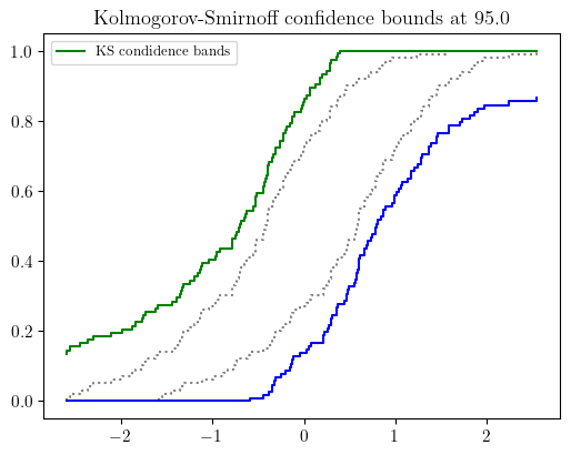
Kolmogorov-Smirnoff confidence bounds illustration with precise and imprecise data.

pyuncertainnumber.fit(method: str, family: str, data: numpy.ndarray) → pyuncertainnumber.UncertainNumber

parametric estimator to fit a distribution from data

Parameters:

• method (str) – method of fitting, e.g., {‘mle’ or ‘mom’} ‘entropy’, ‘pert’, ‘fermi’, ‘bayesian’

• family (str) – distribution family to be fitted

• data (np.ndarray) – data to be fitted

Returns:

• UncertainNumber object

Example

>>> # precise data
>>> pun.fit('mle', 'norm', np.random.normal(0, 1, 100))
>>>  # imprecise data
>>> precise_sample = sps.expon(scale=1/0.4).rvs(15)
>>> imprecise_data = pba.I(lo = precise_sample - 1.4, hi=precise_sample + 1.4)
>>> pun.fit('mom', family='exponential', data=imprecise_data)

See also

pyuncertainnumber.pba.KS_bounds() : a non-parametric charactearisation method using Kolmogorov-Smirnov bounds

class pyuncertainnumber.Pbox(left: numpy.ndarray | list, right: numpy.ndarray | list, steps=Params.steps, mean=None, var=None, p_values=None)

Bases: pyuncertainnumber.pba.mixins.NominalValueMixin, abc.ABC

a base class for Pbox

Danger

this is an abstract class and should not be instantiated directly.

See also

pbox_abc.Staircase and pbox_abc.Leaf for concrete implementations.

property left

property right

steps = 200

mean = None

var = None

_pvalues

abstractmethod _init_moments()

_init_range()

post_init_check()

steps_check()

_compute_nominal_value()

degenerate_flag() → bool

check if the pbox is degenerate (i.e. left == right everywhere)

property degenerate: bool

property p_values

property range

property lo

Returns the left-most value in the interval

property hi

Returns the right-most value in the interval

property support

property median

property enclosed_area

the enclosed area between the two extreme cdfs

__iter__()

__eq__(other)

Equality operator for Pbox objects

Note

• two pboxes are equal if their left and right bounds are equal

__contains__(item)

to_interval()

discretise pbox into a vec-interval of length of default steps

Note

If desired a custom length of vec-interval as output, use discretise() method.

to_dss(discretisation=Params.steps)

convert pbox to DempsterShafer object

to_numpy()

convert pbox to a 2D numpy array (n, 2) of left and right

class pyuncertainnumber.Staircase(left, right, steps=200, mean=None, var=None, p_values=None)

Bases: Pbox

distribution free p-box

_init_moments()

Initialize mean/var interval estimates.

strategy:

1. Try LP-based bounds.

2. If that fails, try ECDF-based bounds.

3. If that also fails, set to NaN intervals so the program continues.

This function NEVER raises.

__repr__()

plot(title=None, ax=None, style='box', fill_color='lightgray', bound_colors=None, bound_styles=None, left_line_kwargs=None, right_line_kwargs=None, nuance='step', alpha=0.3, **kwargs)

default plotting function

Parameters:

• style (str) – ‘box’ or ‘simple’

• fill_color (str) – color to fill the box (only for ‘box’ style)

• bound_colors (list) – list of two colors for left and right bound lines

• bound_styles (list) – list of two linestyles for left and right bound lines

• left_line_kwargs (dict) – additional kwargs for left bound line

• right_line_kwargs (dict) – additional kwargs for right bound line

• nuance (str) – ‘step’ or ‘curve’ for bound line styles

• alpha (float) – transparency level for the box fill (only for ‘box’ style)

• **kwargs – additional keyword arguments for the plot

Note

Two styles are supported: a ‘box’ with fill-in color and a ‘simple’ one without fill-in color. Color and linestyle of the bound lines can be customized via the bound_styles, left_line_kwargs, and right_line_kwargs parameters. The argument nuance controls whether the bound lines are plotted as step functions (‘step’) or smooth curves (‘curve’).

Example

>>> a = pba.normal([2, 6], [0.5, 1])
>>> fig, ax = plt.subplots()
>>> a.plot(ax=ax, style='simple')  # simple style without fill-in color
>>> # box style with fill-in color and also customized bound colors
>>> a.plot(ax=ax, style='box',
...     fill_color='lightblue',
...     bound_colors = ['lightblue', 'lightblue'],
...     bound_styles=("--", ":"),
...     alpha=0.5
... )
>>> # customized left and right bound line styles
>>> ax = pbox.plot(
...     left_line_kwargs={"linestyle": "--", "linewidth": 2},
...     right_line_kwargs={"linestyle": ":", "linewidth": 2, "alpha": 0.8},
)

plot_reverse_axis(title=None, ax=None, style='box', fill_color='lightgray', bound_colors=None, nuance='step', alpha=0.3, orientation='xy', invert_xaxis=True, **kwargs)

A testing plotting function that can swap quantile and probability axes.

Parameters:

• style (str) – ‘box’ or ‘simple’

• orientation (str) – ‘xy’ keeps x on horizontal and Pr(X<=x) on vertical; ‘yx’ swaps them.

plot_outside_legend(title=None, ax=None, style='box', fill_color='lightgray', bound_colors=None, nuance='step', alpha=0.3, **kwargs)

a specific variant of plot() which is used for scipy proceeding only.

Parameters:

style (str) – ‘box’ or ‘simple’

display(*args, **kwargs)

plot_probability_bound(x: float, ax=None, linecolor='r', markercolor='r', **kwargs)

plot the probability bound at a certain quantile x

Note

• a vertical line

plot_quantile_bound(p: float, ax=None, **kwargs)

plot the quantile bound at a certain probability level p

Note

• a horizontal line

classmethod from_CDFbundle(a, b)

pbox from two emipirical CDF bundle

Parameters:

• a (-) – CDF bundle of lower extreme F;

• b (-) – CDF bundle of upper extreme F;

__neg__()

__add__(other)

__radd__(other)

__sub__(other)

__rsub__(other)

__mul__(other)

__rmul__(other)

__truediv__(other)

__rtruediv__(other)

__pow__(other)

__rpow__(other: numbers.Number)

Power operation with the base as other and self as the exponent

__array_ufunc__(ufunc, method, *inputs, **kwargs)

cdf(x: numpy.ndarray)

get the bounds on the cdf w.r.t x value

Parameters:

x (array-like) – x values

alpha_cut(alpha=0.5)

test the lightweight alpha_cut method

Parameters:

alpha (array-like) – probability levels

sample(n_sam)

LHS sampling by default

precise_sample(n_a: int, theta: float = None, n_e: int = None)

Generate precise samples from a p-box

discretise(n=None) → pyuncertainnumber.Interval

alpha-cut discretisation of the p-box without outward rounding

Parameters:

n (int) – number of steps to be used in the discretisation.

Returns:

vector Interval

outer_discretisation(n=None)

discretisation of a p-box to get intervals based on the scheme of outer approximation

Parameters:

n (int) – number of steps to be used in the discretisation

Note

the_interval_list will have length one less than that of default p_values (i.e. 100 and 99)

Returns:

the outer intervals in vec-Interval form

condensation(n) → Self

ourter condensation of the pbox to reduce the number of steps and get a sparser staircase pbox

Parameters:

n (int) – number of steps to be used in the discretisation

Note

Have not thought about a better name so we call it condensation for now. Candidate names include ‘approximation’. It will ouput a p-box and keep steps as 200 for computational consistency.

Example

>>> p.condensation(n=5)

Returns:

a staircase p-box that looks sparser but has the same number of steps

condense(n) → pyuncertainnumber.pba.dss.DempsterShafer

Another condensation function which has steps of n

Compared to the above condensation method that ouputs a p-box and keeps steps as 200 for computational consistency. This one condenses in a more literal manner, as in having n steps in the resulting Dempster-Shafer structure.

truncate(a, b)

Truncate the Pbox to the range [a, b].

example: >>> from pyuncertainnumber import pba >>> p = pba.normal([4, 9], 1) >>> tr = p.truncate(3, 8) >>> fig, ax = plt.subplots() >>> p.plot(ax=ax) >>> tr.plot(ax=ax, fill_color=’r’) >>> plt.show()

min(other, method='f')

Returns a new Pbox object that represents the element-wise minimum of two Pboxes.

Parameters:

• other (-) – Another Pbox object or a numeric value.

• method (-) – Calculation method to determine the minimum. Can be one of ‘f’, ‘p’, ‘o’, ‘i’.

Returns:

Pbox

max(other, method='f')

get_PI(alpha: numbers.Number = 0.95, style='narrowest') → pyuncertainnumber.Interval

Compute the predictive interval at the coverage level of alpha

Parameters:

• alpha (Number) – coverage level for the predictive interval, default is 0.95

• style (str) – ‘narrowest’ or ‘widest’, default is ‘narrowest’

Note

by default, narrowest predictive interval is returned; when the narrowest does not exist, a warning will the generated and then the widest is returned instead.

Example

>>> from pyuncertainnumber import pba
>>> p = pba.normal([10, 15, 1])
>>> p.get_PI(alpha=0.95, style='narrowest')

straddles(N, endpoints=True) → bool

Check whether the p-box straddles a number N

Parameters:

• N (float) – the Number to check

• endpoints (Boolean) – Whether to include the endpoints within the check

Returns:

True

If \(\mathrm{left} \leq N \leq \mathrm{right}\) (Assuming endpoints=True)

False

Otherwise

Note

This could affect the results of Frechet bounds

straddles_zero() → bool

Checks specifically whether \(0\) is within the p-box

is_zero()

is_nagative()

env(other)

computes the envelope of two Pboxes.

Parameters:

other (Pbox)

Returns:

• Pbox

imp(other)

Returns the imposition of self with other pbox

Note

• binary imposition between two pboxes only

_unary_template(f)

exp()

exponential function: e^x

sqrt()

square root function: √x

reciprocal()

Calculate the reciprocal of the pbox

Note

the pbox should not straddle zero, otherwise a warning is raised

log()

natural logarithm of the pbox

Note

• the pbox must be positive

sin()

cos()

tanh()

add(other, dependency='f')

sub(other, dependency='f')

mul(other, dependency='f')

Multiplication of uncertain numbers with the defined dependency dependency

div(other, dependency='f')

pow(other, dependency='f')

Exponentiation of uncertain numbers with the defined dependency dependency

This suggests that the exponent (i.e. other) can also be an uncertain number.

balchprod(other)

Frechet convolution of two pboxes when any of them straddles zero

class pyuncertainnumber.Interval(lo: float | numpy.ndarray, hi: float | numpy.ndarray | None = None, do_heavy_checks: bool = True)

Bases: pyuncertainnumber.pba.mixins.NominalValueMixin

Interval is the main class

_lo

_hi = None

run_heavy_checks()

Run heavy checks on the interval object

__repr__()

__str__()

__len__()

__iter__()

__contains__(item)

Check if an item is enclosed within the interval.

Example

>>> i = Interval(1,3)
>>> 2 in i
True
>>> 4 in i
False

__next__()

__getitem__(i: int | slice)

to_numpy() → numpy.ndarray

transform interval objects to numpy arrays

to_pbox()

lhs_sample(n) → numpy.ndarray

LHS sampling within the interval

Parameters:

n – number of samples

endpoints_lhs_sample(n) → numpy.ndarray

LHS sampling within the interval plus the endpoints

Parameters:

n – number of samples

plot(ax=None, **kwargs)

display()

is_degenerate() → bool

Check if the interval is degenerate (i.e., has zero width).

_compute_nominal_value()

ravel()

Return a flattened (1D) interval object for multi-dimensional intervals

Example

>>> A = np.random.rand(200, 200, 2)
>>> i = pba.intervalise(A)
>>> print(i.shape)
>>> i2 = i.ravel()
>>> print(i2.shape)

property lo: numpy.ndarray | float

property hi: numpy.ndarray | float

property left

property right

property width

property rad

half width

property mid

property unsized

property val

seemingly equivalent to self.to_numpy()

property scalar

Check if the interval is wide sense scalar

Note

wide sense: I(1,2) and I([1],[2]) are both scalars

property is_scalar

Check if the interval is a strict-sense scalar

Note

strict sense: I(1,2) is a scalar, but I([1],[2]) is not

property shape

property ndim

__neg__()

__pos__()

__add__(other)

__radd__(left)

__sub__(other)

__rsub__(left)

__mul__(other)

__rmul__(left)

__truediv__(other)

__rtruediv__(left)

__pow__(other)

__lt__(other)

__rlt__(left)

__gt__(other)

__rgt__(left)

__le__(other)

__rle__(left)

__ge__(other)

__rge__(left)

__eq__(other)

__ne__(other)

__array_ufunc__(ufunc, method, *inputs, **kwargs)

abs()

sqrt()

exp()

log()

sin()

cos()

tan()

classmethod from_meanform(x, half_width)

save_json(filename: str, comment: str = None, save_dir: str | pathlib.Path = '.') → None

Save the interval object to a JSON5 file.

Parameters:

• filename (str) – The name of the file (without extension) to save the interval object to.

• comment (str, optional) – A comment to include at the top of the file.

• save_dir (str | Path, optional) – Directory where the file should be saved. Defaults to current directory.

Note

The file is saved with a .json5 extension.

Example

>>> a.save_json("interval_data", comment="This is interval data", save_dir="results/")

pyuncertainnumber.make_vec_interval(vec)

parse an array-like structure into a vector interval

For most part, it works same to intervalise, except that this function can also handle a list of UN objects.

Example

>>> a, b = pba.I(1, 2), pba.I(3, 4)
>>> make_vec_interval([a, b])
Interval([1, 3], [2, 4])

pyuncertainnumber.parse_bounds(b)

top-level function that universally parses scalar and vector bounds

pyuncertainnumber.intervalise(x_: Any, interval_index=-1) → pyuncertainnumber.pba.intervals.number.Interval | Any

This function casts an array-like structure into an Interval structure. All array-like structures will be first coerced into an ndarray of floats. If the coercion is unsuccessful the following error is thrown: ValueError: setting an array element with a sequence.

For example this is the expected behaviour: (*) an ndarray of shape (4,2) will be cast as an Interval of shape (4,).

(*) an ndarray of shape (7,3,2) will be cast as an Interval of shape (7,3).

(*) an ndarray of shape (3,2,7) will be cast as a degenerate Interval of shape (3,2,7).

(*) an ndarray of shape (2,3,7) will be cast as an Interval of shape (3,7).

(*) an ndarray of shape (2,3,7,2) will be cast as an Interval of shape (2,3,7) if interval_index is set to -1.

If an ndarray has shape with multiple dimensions having size 2, then the last dimension is intervalised. So, an ndarray of shape (7,2,2) will be cast as an Interval of shape (7,2) with the last dimension intervalised. When the ndarray has shape (2,2) again is the last dimension that gets intervalised.

In case of ambiguity, e.g. (2,5,2), now the first dimension can be forced to be intervalised, selecting index=0, default is -1.

It returns an interval only if the input is an array-like structure, otherwise it returns the following numpy error: ValueError: setting an array element with a sequence.

TODO: Parse a list of mixed numbers: interval and ndarrays.

class pyuncertainnumber.EpistemicDomain(*vars: pyuncertainnumber.pba.intervals.Interval)

Representation of the epistemic space which are indeed bounds of each dimension

This class provides a set of handy functions to work with epistemic uncertainty in the form of bounds. It will be useful for tasks such as propagation or optimization where epistemic uncertainty is involved.

Parameters:

vars – a set of Interval variables

Tip

Recommended to use for optimisation tasks where the design bounds can be quickly specified with the toOptBounds() method.

See also

pyuncertainnumber.src.pyuncertainnumber.opt.bo : Bayesian optimisation class.

pyuncertainnumber.src.pyuncertainnumber.opt.ga : Genetic algorithm class.

Example

>>> from pyuncertainnumber import pba
>>> e = EpistemicDomain(pba.I(-1, 3), pba.I(5, 9))

>>> # convert the epistemic space to bounds for the optimizer
>>> e.toOptBounds(method='GA')  # `varbound` for genetic algorithm
>>> e.toOptBounds(method='BO')  # `xc_bounds` for Bayesian optimisation

>>> # perform lhs sampling on the epistemic space
>>> sample = e.lhs_sampling(1000)

lhs_sampling(n_samples: int)

perform lhs sampling on the epistemic space

lhs_plus_endpoints(n_samples: int)

perform lhs sampling on the epistemic space and add endpoints

bound_rep()

return the bounds (vec or matrix) of the epistemic space

toOptBounds(method: str)

convert the epistemic space to bounds for the optimizer

Parameters:

method (str) – the optimization method to use, e.g. ‘BayesOpt’, ‘GA’

Returns:

the bounds of the design varibale used for the optimisation method

to_GA_varBounds() → numpy.ndarray

convert the epistemic space to bounds for the genetic algorithm optimizer

to_BayesOptBounds(func_signature='vectorisation') → dict

convert the epistemic space to bounds for the Bayesian optimisation optimizer

pyuncertainnumber.hedge_interpret(hedge: str, return_type='interval') → pyuncertainnumber.pba.intervals.Interval | pyuncertainnumber.pba.pbox_abc.Pbox

interpret linguistic hedge words into UncertainNumber objects

Parameters:

• hedge (str) – the hedge numerical expression to be interpreted

• return_type (str) – the type of object to be returned, either ‘interval’ or ‘pbox’

Note

• the return can either be an interval or a pbox object

Example

>>> hedge_interpret("about 200", return_type="pbox")
>>> hedge_interpret("200.00")

pyuncertainnumber.infer_cbox(family: str, data, **args) → pyuncertainnumber.pba.cbox_constructor.Cbox

top-level call signature to infer a c-box given data and family, plus rarely additional kwargs

Notes

• data (list): a list of data samples, e.g. [2]

• additina kwargs such as N for binomial family

Example

>>> infer_cbox('binomial', data=[2], N=10)

pyuncertainnumber.infer_predictive_distribution(family: str, data, **args)

top-level call for the next value predictive distribution

class pyuncertainnumber.dempstershafer_element

Bases: tuple

interval

mass

class pyuncertainnumber.DempsterShafer(intervals: pyuncertainnumber.pba.intervals.Interval | list[list] | list[pyuncertainnumber.pba.intervals.Interval] | numpy.ndarray, masses: numpy.typing.ArrayLike)

Bases: pyuncertainnumber.pba.mixins.NominalValueMixin, pyuncertainnumber.pba.mixins._PboxOpsMixin

Class for Dempester-Shafer structures.

Parameters:

• intervals – expect wildcard vector intervals, vec-Interval; list of scalar intervals; list of list pairs; or 2D array;

• masses (ArrayLike) – probability masses

Example

>>> from pyuncertainnumber import pba
>>> dss = pba.DempsterShafer(intervals=[[1,5], [3,6]], masses=[0.5, 0.5])
>>> dss.structures
[dempstershafer_element(interval=[1.0,5.0], mass=0.5),
 dempstershafer_element(interval=[3.0,6.0], mass=0.5)]

Note

Dempster-Shafer structures are also called belief structures or evidence structures, and it can be converted to p-boxes.

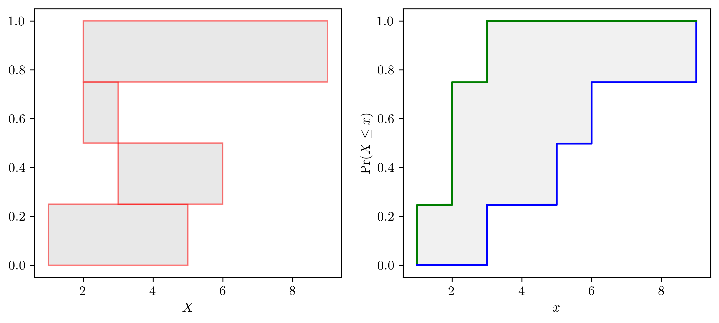
P-box and Dempster Shafer structure illustration.

_intervals

_masses

_create_DSstructure()

__repr__()

_compute_nominal_value()

property structures

property intervals

Returns the Interval-typed focal elements of the Dempster-Shafer structure.

property focal_elements

Returns the focal elements of the Dempster-Shafer structure.

property masses

plot(style='raw', ax=None, zorder=None, **kwargs)

for box type transform dss into a pbox and plot

Parameters:

• style (str) – “raw” (default), “box”, “pbox”, “interval”

• edge_color (str) – edge color for raw style. If None, use default red color.

display(style='box', ax=None, **kwargs)

to_pbox()

_to_pbox()

for mixin use only

classmethod from_dsElements(*ds_elements: dempstershafer_element)

Create a Dempster-Shafer structure from a list of Dempster-Shafer elements.

class pyuncertainnumber.Dependency(family: str, params: numbers.Number | None = None, **kwargs)

Dependency class to specify copula models.

Parameters:

• family (str) – Name of the copula family, one of “gaussian”, “t”, “frank”, “gumbel”, “clayton”, “independence”.

• params (Number | None) – Backward-compatible single-parameter shortcut: - gaussian/t: interpreted as corr - frank/gumbel/clayton: interpreted as theta - independence: ignored

• **kwargs – Any keyword parameters supported by the selected copula, e.g. corr=…, df=…, theta=…, k_dim=…, allow_singular=…

Examples

>>> Dependency("gaussian", params=0.8, k_dim=3)          # legacy style
>>> Dependency("gaussian", corr=0.8, k_dim=3)            # explicit
>>> Dependency("t", corr=0.6, df=5, k_dim=4)
>>> Dependency("frank", theta=2.5, k_dim=2)
>>> Dependency("independence", k_dim=5)

copulas_dict

_single_param_alias

family = ''

params = None

_copula

property copula

Access the underlying statsmodels copula instance.

_post_init_check()

__repr__()

pdf(u)

cdf(u)

u_sample(n: int, random_state=None)

draws n samples in the U space (unit hypercube)

display(style='3d_cdf', ax=None)

show the PDF or CDF in the u space

fit(data)

pyuncertainnumber.KS_bounds(s: numpy.typing.ArrayLike, alpha: float, display=True, output_type='bounds') → tuple[pyuncertainnumber.pba.ecdf.eCDF_bundle] | pyuncertainnumber.pba.pbox_abc.Pbox | pyuncertainnumber.UncertainNumber

construct free pbox from sample data by Kolmogorov-Smirnoff confidence bounds

Parameters:

• s (ArrayLike) – sample data, precise and imprecise

• dn (float) – KS critical value at a significance level and sample size N;

• output_type (str) – A choice between {‘bounds’, ‘pbox’, ‘un’}, default=’bounds’ which returns two eCDF bundles as bounds; ‘pbox’ to return a pbox object; ‘un’ to return an uncertain number object.

Returns:

a tuple of two CDF bounds, i.e. upper and lower (eCDF_bundle objects), or a Pbox object, or an UncertainNumber object the return type is controlled by the output_type argument.

Note

By default the function returns two eCDF bundles as the extreme bounds. With the upper and lower bounds, a free pbox can be constructed.

Example

>>> # both precise data (e.g. numpy array) and imprecise data (e.g. a vector of interval) are supported
>>> precise_data = np.random.normal(0, 1, 100)  # precise data case
>>> ub, lb = pba.KS_bounds(precise_data, alpha=0.025, display=True)

>>> # alternatively, an uncertain number or a p-box can be returned
>>> pba.KS_bounds(precise_data, alpha=0.025, display=False, output_type='pbox')  # return a pbox object
>>> pba.KS_bounds(precise_data, alpha=0.025, display=False, output_type='un')  # return an uncertain number object

>>> # imprecise data case
>>> impre_data = pba.I(lo = precise_data -0.5, hi = precise_data + 0.5)
>>> ub, lb = pba.KS_bounds(impre_data, alpha=0.025, display=True)

Kolmogorov-Smirnoff confidence bounds illustration with precise and imprecise data.

pyuncertainnumber.make_vec_interval(vec)

parse an array-like structure into a vector interval

For most part, it works same to intervalise, except that this function can also handle a list of UN objects.

Example

>>> a, b = pba.I(1, 2), pba.I(3, 4)
>>> make_vec_interval([a, b])
Interval([1, 3], [2, 4])

pyuncertainnumber.reweighting(*masses)

reweight the masses to sum to 1

class pyuncertainnumber.eCDF_bundle

a handy tuple of eCDF function q and p

quantiles: numpy.ndarray

probabilities: numpy.ndarray

__repr__()

classmethod from_sps_ecdf(e)

utility to tranform sps.ecdf to eCDF_bundle

plot_bounds(other)

plot the lower and upper bounds

pyuncertainnumber.get_ecdf(s, w=None, display=False) → tuple

compute the weighted ecdf from (precise) sample data

Parameters:

• s (array-like) – 1 dimensional precise sample data

• w (array-like) – weights

Note

• Sudret eq.1

Returns:

ecdf in the form of a tuple of q and p

class pyuncertainnumber.Interval(lo: float | numpy.ndarray, hi: float | numpy.ndarray | None = None, do_heavy_checks: bool = True)

Bases: pyuncertainnumber.pba.mixins.NominalValueMixin

Interval is the main class

_lo

_hi = None

run_heavy_checks()

Run heavy checks on the interval object

__repr__()

__str__()

__len__()

__iter__()

__contains__(item)

Check if an item is enclosed within the interval.

Example

>>> i = Interval(1,3)
>>> 2 in i
True
>>> 4 in i
False

__next__()

__getitem__(i: int | slice)

to_numpy() → numpy.ndarray

transform interval objects to numpy arrays

to_pbox()

lhs_sample(n) → numpy.ndarray

LHS sampling within the interval

Parameters:

n – number of samples

endpoints_lhs_sample(n) → numpy.ndarray

LHS sampling within the interval plus the endpoints

Parameters:

n – number of samples

plot(ax=None, **kwargs)

display()

is_degenerate() → bool

Check if the interval is degenerate (i.e., has zero width).

_compute_nominal_value()

ravel()

Return a flattened (1D) interval object for multi-dimensional intervals

Example

>>> A = np.random.rand(200, 200, 2)
>>> i = pba.intervalise(A)
>>> print(i.shape)
>>> i2 = i.ravel()
>>> print(i2.shape)

property lo: numpy.ndarray | float

property hi: numpy.ndarray | float

property left

property right

property width

property rad

half width

property mid

property unsized

property val

seemingly equivalent to self.to_numpy()

property scalar

Check if the interval is wide sense scalar

Note

wide sense: I(1,2) and I([1],[2]) are both scalars

property is_scalar

Check if the interval is a strict-sense scalar

Note

strict sense: I(1,2) is a scalar, but I([1],[2]) is not

property shape

property ndim

__neg__()

__pos__()

__add__(other)

__radd__(left)

__sub__(other)

__rsub__(left)

__mul__(other)

__rmul__(left)

__truediv__(other)

__rtruediv__(left)

__pow__(other)

__lt__(other)

__rlt__(left)

__gt__(other)

__rgt__(left)

__le__(other)

__rle__(left)

__ge__(other)

__rge__(left)

__eq__(other)

__ne__(other)

__array_ufunc__(ufunc, method, *inputs, **kwargs)

abs()

sqrt()

exp()

log()

sin()

cos()

tan()

classmethod from_meanform(x, half_width)

save_json(filename: str, comment: str = None, save_dir: str | pathlib.Path = '.') → None

Save the interval object to a JSON5 file.

Parameters:

• filename (str) – The name of the file (without extension) to save the interval object to.

• comment (str, optional) – A comment to include at the top of the file.

• save_dir (str | Path, optional) – Directory where the file should be saved. Defaults to current directory.

Note

The file is saved with a .json5 extension.

Example

>>> a.save_json("interval_data", comment="This is interval data", save_dir="results/")

class pyuncertainnumber.Staircase(left, right, steps=200, mean=None, var=None, p_values=None)

Bases: Pbox

distribution free p-box

_init_moments()

Initialize mean/var interval estimates.

strategy:

1. Try LP-based bounds.

2. If that fails, try ECDF-based bounds.

3. If that also fails, set to NaN intervals so the program continues.

This function NEVER raises.

__repr__()

plot(title=None, ax=None, style='box', fill_color='lightgray', bound_colors=None, bound_styles=None, left_line_kwargs=None, right_line_kwargs=None, nuance='step', alpha=0.3, **kwargs)

default plotting function

Parameters:

• style (str) – ‘box’ or ‘simple’

• fill_color (str) – color to fill the box (only for ‘box’ style)

• bound_colors (list) – list of two colors for left and right bound lines

• bound_styles (list) – list of two linestyles for left and right bound lines

• left_line_kwargs (dict) – additional kwargs for left bound line

• right_line_kwargs (dict) – additional kwargs for right bound line

• nuance (str) – ‘step’ or ‘curve’ for bound line styles

• alpha (float) – transparency level for the box fill (only for ‘box’ style)

• **kwargs – additional keyword arguments for the plot

Note

Two styles are supported: a ‘box’ with fill-in color and a ‘simple’ one without fill-in color. Color and linestyle of the bound lines can be customized via the bound_styles, left_line_kwargs, and right_line_kwargs parameters. The argument nuance controls whether the bound lines are plotted as step functions (‘step’) or smooth curves (‘curve’).

Example

>>> a = pba.normal([2, 6], [0.5, 1])
>>> fig, ax = plt.subplots()
>>> a.plot(ax=ax, style='simple')  # simple style without fill-in color
>>> # box style with fill-in color and also customized bound colors
>>> a.plot(ax=ax, style='box',
...     fill_color='lightblue',
...     bound_colors = ['lightblue', 'lightblue'],
...     bound_styles=("--", ":"),
...     alpha=0.5
... )
>>> # customized left and right bound line styles
>>> ax = pbox.plot(
...     left_line_kwargs={"linestyle": "--", "linewidth": 2},
...     right_line_kwargs={"linestyle": ":", "linewidth": 2, "alpha": 0.8},
)

plot_reverse_axis(title=None, ax=None, style='box', fill_color='lightgray', bound_colors=None, nuance='step', alpha=0.3, orientation='xy', invert_xaxis=True, **kwargs)

A testing plotting function that can swap quantile and probability axes.

Parameters:

• style (str) – ‘box’ or ‘simple’

• orientation (str) – ‘xy’ keeps x on horizontal and Pr(X<=x) on vertical; ‘yx’ swaps them.

plot_outside_legend(title=None, ax=None, style='box', fill_color='lightgray', bound_colors=None, nuance='step', alpha=0.3, **kwargs)

a specific variant of plot() which is used for scipy proceeding only.

Parameters:

style (str) – ‘box’ or ‘simple’

display(*args, **kwargs)

plot_probability_bound(x: float, ax=None, linecolor='r', markercolor='r', **kwargs)

plot the probability bound at a certain quantile x

Note

• a vertical line

plot_quantile_bound(p: float, ax=None, **kwargs)

plot the quantile bound at a certain probability level p

Note

• a horizontal line

classmethod from_CDFbundle(a, b)

pbox from two emipirical CDF bundle

Parameters:

• a (-) – CDF bundle of lower extreme F;

• b (-) – CDF bundle of upper extreme F;

__neg__()

__add__(other)

__radd__(other)

__sub__(other)

__rsub__(other)

__mul__(other)

__rmul__(other)

__truediv__(other)

__rtruediv__(other)

__pow__(other)

__rpow__(other: numbers.Number)

Power operation with the base as other and self as the exponent

__array_ufunc__(ufunc, method, *inputs, **kwargs)

cdf(x: numpy.ndarray)

get the bounds on the cdf w.r.t x value

Parameters:

x (array-like) – x values

alpha_cut(alpha=0.5)

test the lightweight alpha_cut method

Parameters:

alpha (array-like) – probability levels

sample(n_sam)

LHS sampling by default

precise_sample(n_a: int, theta: float = None, n_e: int = None)

Generate precise samples from a p-box

discretise(n=None) → pyuncertainnumber.Interval

alpha-cut discretisation of the p-box without outward rounding

Parameters:

n (int) – number of steps to be used in the discretisation.

Returns:

vector Interval

outer_discretisation(n=None)

discretisation of a p-box to get intervals based on the scheme of outer approximation

Parameters:

n (int) – number of steps to be used in the discretisation

Note

the_interval_list will have length one less than that of default p_values (i.e. 100 and 99)

Returns:

the outer intervals in vec-Interval form

condensation(n) → Self

ourter condensation of the pbox to reduce the number of steps and get a sparser staircase pbox

Parameters:

n (int) – number of steps to be used in the discretisation

Note

Have not thought about a better name so we call it condensation for now. Candidate names include ‘approximation’. It will ouput a p-box and keep steps as 200 for computational consistency.

Example

>>> p.condensation(n=5)

Returns:

a staircase p-box that looks sparser but has the same number of steps

condense(n) → pyuncertainnumber.pba.dss.DempsterShafer

Another condensation function which has steps of n

Compared to the above condensation method that ouputs a p-box and keeps steps as 200 for computational consistency. This one condenses in a more literal manner, as in having n steps in the resulting Dempster-Shafer structure.

truncate(a, b)

Truncate the Pbox to the range [a, b].

example: >>> from pyuncertainnumber import pba >>> p = pba.normal([4, 9], 1) >>> tr = p.truncate(3, 8) >>> fig, ax = plt.subplots() >>> p.plot(ax=ax) >>> tr.plot(ax=ax, fill_color=’r’) >>> plt.show()

min(other, method='f')

Returns a new Pbox object that represents the element-wise minimum of two Pboxes.

Parameters:

• other (-) – Another Pbox object or a numeric value.

• method (-) – Calculation method to determine the minimum. Can be one of ‘f’, ‘p’, ‘o’, ‘i’.

Returns:

Pbox

max(other, method='f')

get_PI(alpha: numbers.Number = 0.95, style='narrowest') → pyuncertainnumber.Interval

Compute the predictive interval at the coverage level of alpha

Parameters:

• alpha (Number) – coverage level for the predictive interval, default is 0.95

• style (str) – ‘narrowest’ or ‘widest’, default is ‘narrowest’

Note

by default, narrowest predictive interval is returned; when the narrowest does not exist, a warning will the generated and then the widest is returned instead.

Example

>>> from pyuncertainnumber import pba
>>> p = pba.normal([10, 15, 1])
>>> p.get_PI(alpha=0.95, style='narrowest')

straddles(N, endpoints=True) → bool

Check whether the p-box straddles a number N

Parameters:

• N (float) – the Number to check

• endpoints (Boolean) – Whether to include the endpoints within the check

Returns:

True

If \(\mathrm{left} \leq N \leq \mathrm{right}\) (Assuming endpoints=True)

False

Otherwise

Note

This could affect the results of Frechet bounds

straddles_zero() → bool

Checks specifically whether \(0\) is within the p-box

is_zero()

is_nagative()

env(other)

computes the envelope of two Pboxes.

Parameters:

other (Pbox)

Returns:

• Pbox

imp(other)

Returns the imposition of self with other pbox

Note

• binary imposition between two pboxes only

_unary_template(f)

exp()

exponential function: e^x

sqrt()

square root function: √x

reciprocal()

Calculate the reciprocal of the pbox

Note

the pbox should not straddle zero, otherwise a warning is raised

log()

natural logarithm of the pbox

Note

• the pbox must be positive

sin()

cos()

tanh()

add(other, dependency='f')

sub(other, dependency='f')

mul(other, dependency='f')

Multiplication of uncertain numbers with the defined dependency dependency

div(other, dependency='f')

pow(other, dependency='f')

Exponentiation of uncertain numbers with the defined dependency dependency

This suggests that the exponent (i.e. other) can also be an uncertain number.

balchprod(other)

Frechet convolution of two pboxes when any of them straddles zero

pyuncertainnumber.convert(un)

Convert any input un into a Pbox object

Note

• theorically ‘un’ can be {Interval, DempsterShafer, Distribution, float, int}

class pyuncertainnumber.Params

steps = 200

many = 2000

p_lboundary = 0.001

p_hboundary = 0.999

p_values

scott_hedged_interpretation

user_hedged_interpretation

pyuncertainnumber.envelope(*l_uns: pyuncertainnumber.pba.pbox_abc.Pbox | pyuncertainnumber.pba.dss.DempsterShafer | numbers.Number | pyuncertainnumber.pba.intervals.Interval | pyuncertainnumber.pba.distributions.Distribution | pyuncertainnumber.characterisation.uncertainNumber.UncertainNumber, output_type='pbox') → pyuncertainnumber.pba.pbox_abc.Staircase | pyuncertainnumber.characterisation.uncertainNumber.UncertainNumber

calculates the envelope of constructs only

Parameters:

• l_uns (list) – the components, constructs and uncertain numbers, on which the envelope operation applied on.

• output_type (str) – {‘pbox’ or ‘uncertain_number’ or ‘un’} - default is pbox

Returns:

the envelope of the given arguments, either a p-box or an interval.

Example

>>> from pyuncertainnumber import envelope
>>> a = pba.normal(3, 1)
>>> b = pba.uniform(5, 8)
>>> c = pba.normal(13, 2)
>>> t = envelope(a, b, c, output_type='pbox') # or output_type='uncertain_number'

pyuncertainnumber.imposition(*l_uns: pyuncertainnumber.pba.pbox_abc.Pbox | pyuncertainnumber.pba.dss.DempsterShafer | numbers.Number | pyuncertainnumber.pba.intervals.Interval | pyuncertainnumber.pba.distributions.Distribution | pyuncertainnumber.characterisation.uncertainNumber.UncertainNumber, output_type='pbox') → pyuncertainnumber.pba.pbox_abc.Staircase | pyuncertainnumber.characterisation.uncertainNumber.UncertainNumber

Returns the imposition/intersection of the list of p-boxes

Parameters:

• l_uns (list) – a list of constructs or UN objects to be mixed

• output_type (str) – {‘pbox’ or ‘uncertain_number’ or ‘un’} - default is pbox

Returns:

• Pbox or UncertainNumber

Example

>>> import pyuncertainnumber as pun
>>> from pyuncertainnumber import pba
>>> a = pba.normal([3, 7], 1)
>>> b = pba.uniform([3,5], [6,9])
>>> i = pun.imposition(a, b)

pyuncertainnumber.stochastic_mixture(*l_uns: pyuncertainnumber.pba.pbox_abc.Pbox | pyuncertainnumber.pba.dss.DempsterShafer | numbers.Number | pyuncertainnumber.pba.intervals.Interval | pyuncertainnumber.pba.distributions.Distribution | pyuncertainnumber.characterisation.uncertainNumber.UncertainNumber, weights=None)

it could work for either Pbox, distribution, DS structure or Intervals

Parameters:

• l_uns (-) – list of constructs or uncertain numbers

• weights (-) – list of weights

Example

>>> import pyuncertainnumber as pun
>>> p = pun.stochastic_mixture([[1,3], [2,4]])

pyuncertainnumber.stacking(vec_interval: pyuncertainnumber.pba.intervals.Interval | list[pyuncertainnumber.pba.intervals.Interval], *, weights=None, display=False, ax=None, return_type='pbox', **kwargs) → pyuncertainnumber.pba.pbox_abc.Pbox

stochastic mixture operation of Intervals with probability masses

Parameters:

• vec_interval (-) – list of Intervals or a vectorised Interval

• weights (-) – list of weights

• display (-) – boolean for plotting

• return_type (-) – {‘pbox’ or ‘ds’ or ‘bounds’}

Returns:

by default a p-box but can return the left and right bound F in eCDF_bundlebounds.

Note

• For intervals specifically.

• it takes a list of intervals or a single vectorised interval, which is

a different signature compared to the other aggregation functions. - together the interval and masses, it can be deemed that all the inputs required is jointly a DS structure

Example

>>> stacking([[1,3], [2,4]], weights=[0.5, 0.5], display=True)

pyuncertainnumber.mixture_pbox(*l_pboxes, weights=None, display=False) → pyuncertainnumber.pba.pbox_abc.Pbox

pyuncertainnumber.mixture_ds(*l_ds, display=False) → pyuncertainnumber.pba.dss.DempsterShafer

mixture operation for DS structure

pyuncertainnumber.env_samples(data: numpy.typing.ArrayLike, output_type='pbox', ecdf_choice='canonical')

nonparametric envelope function directly from data samples

Parameters:

• data (ArrayLike) – Each row represents a distribution, on which the envelope operation applied.

• output_type (str) – {‘pbox’ or ‘cdf’} default is pbox cdf is the CDF bundle

• ecdf_choice (str) – {‘canonical’ or ‘staircase’}

Note

envelope on a set of empirical CDFs

pyuncertainnumber.env_ecdf_sep(*ecdfs, output_type='pbox', ecdf_choice='canonical')

nonparametric envelope function for separate empirical CDFs

pyuncertainnumber.env_am(n_pars: numpy.typing.ArrayLike) → numpy.ndarray

bespoke function used for am metric case

Parameters:

n_pars (ArrayLike) – (n_sam, 2) of tuple (mu, sigma) which may be a tensor

pyuncertainnumber.env_pbox_am(n_mean: numpy.typing.ArrayLike, n_std: numpy.typing.ArrayLike) → numpy.ndarray

bespoke function used for am metric case

Parameters:

• n_mean (ArrayLike) – (n_sam,) of mean values which may be a tensor

• n_std (ArrayLike) – (n_sam,) of standard deviation values which may be a tensor

pyuncertainnumber.b2b(vars: pyuncertainnumber.pba.intervals.number.Interval | list[pyuncertainnumber.pba.intervals.number.Interval], func: callable, interval_strategy: str = None, subinterval_style: str = None, n_sub: int = None, n_sam: int = 200, **kwargs) → pyuncertainnumber.pba.intervals.number.Interval

General implementation of interval propagation through a function:

\[Y = g(I_{x1}, I_{x2}, ..., I_{xn})\]

where \(I_{x1}, I_{x2}, ..., I_{xn}\) are intervals.

In a general case, the function \(g\) is not necessarily monotonic and \(g\) may be a black-box model. Optimisation to the rescue and two of them particularly: Genetic Algorithm and Bayesian Optimisation.

Parameters:

• vars (Interval | list[Interval]) – a vector Interval or a list or tuple of scalar Intervals, or an EpistemicDomain object, or a scalar Interval;

• func (callable) – performance or response function or a black-box model as in subprocess. Expect 2D inputs therefore func shall have the matrix signature. See Notes for additional details.

• interval_strategy (str) –

  the interval_strategy used for interval propagation. The choice shall be compatible with the response function signature. Seethe notes below for additional details.

  • ’endpoints’: only the endpoints

  • ’ga’: genetic algorithm

  • ’bo’: bayesian optimisation

  • ’direct’: directly apply function to the input intervals (the default)

  • ’subinterval’: apply function to subintervals

  • ’cauchy_deviate’: use the Cauchy Deviate Method for interval propagation

• subinterval_style (str) – the subinterval_style only used for subinterval propagation, including {‘’direct’’, ‘’endpoints’’}.

• n_sub (int) – number of subintervals, only used for subinterval propagation.

• n_sam (int) – number of samples, only used for Cauchy deviate method

• **kwargs – additional keyword arguments to be passed to the function, which provides extra control for the algorithm used. For example, for GA, one can pass in ‘algorithm_param’ for BO, one can pass in ‘acquisition_function’, ‘num_iterations’ etc. Typically, one would try the optimisation harder (e.g. more iterations) for a more accurate result.

Tip

This serves as a top-level for generic interval propagation .

Caution

interval_strategy suggests the method of interval propagation (e.g. ‘direct’ or ‘endpoints’, or ‘subinterval’, or ‘ga’, or ‘bo’), whhile subinterval_style is only used for ‘subinterval’ propagation. This is to say that what strategy (whether ‘direct’ or ‘endpoints’) will be further chosen for the sub-intervals. For scalar function propagation, vars shuld just be a scalar Interval object rather than a list.

Danger

There are some subtleties about the calling signature of the propagating function. For endpoints strategy/subinterval_style, the function func should have a vectorised signature as it is expecting a 2D numpy array, whereas for the direct strategy/subinterval_style, it is expecting to take individual scalar inputs. It is recommended to write a function which implements both signature, as seen in the example below.

Returns:

the low and upper bound of the response

Return type:

Interval

Example

>>> from pyuncertainnumber import b2b
>>> import numpy as np
>>> import pyuncertainnumber as pba

>>> # Define a universal function that handles a performance function with both `vectorised` and `iterable` signatures
>>> def bar_universal(x):
...     if isinstance(x, np.ndarray):  # foo_vectorised signature
...         if x.ndim == 1:
...             x = x[None, :]
...         return x[:, 0] ** 3 + x[:, 1] + 5
...     else:
...         return x[0] ** 3 + x[1] + 5  # foo_iterable signature

>>> # Define input intervals
>>> a = pba.I(3., 5.)
>>> b = pba.I(6., 26.)

>>> # using the {'endpoints', "direct", ga", "bo"} strategy
>>> b2b(vars=[a, b],
...     func=bar_universal,
...     interval_strategy='endpoints')  # replace with {"direct", ga", "bo"}

>>> # using the 'subinterval' strategy
>>> b2b(vars=[a, b],
...     func=bar_universal,
...     interval_strategy='subinterval',
...     subinterval_style='endpoints',
...     n_sub=2)

>>> # using the 'cauchy_deviate' strategy
>>> b2b(vars=[a, b],
...     func=bar_universal,
...     interval_strategy='cauchy_deviate',
...     n_sam=1000)

>>> # in comparison, one can compare with the result of interval arithmetic
>>> def bar_individual(x1, x2):
...     return x1 ** 3 + x2 + 5  # individual signature
>>> bar_individual(a, b)
[38.0, 156.0]

class pyuncertainnumber.Propagation(vars: list[pyuncertainnumber.characterisation.uncertainNumber.UncertainNumber], func: callable, method: str, dependency: str | pyuncertainnumber.pba.dependency.Dependency = None, interval_strategy: str = None)

High-level integrated class for the propagation of uncertain numbers

Parameters:

• vars (UncertainNumber) – a list of uncertain numbers objects

• func (Callable) – the response or performance function applied to the uncertain numbers

• method (str) – a string indicating the method to be used for propagation (e.g. “monte_carlo”, “endpoint”, etc.) which may depend on the constructs of the uncertain numbers. See notes about function signature.

• dependency (string or Dependency) – a Dependency object(i.e. a copula function) to model the dependency structure among input variables. Strings such as “independence” accepted for independence.

• interval_strategy (str) – a strategy for interval propagation, including {‘direct’, ‘subinterval’, ‘endpoints’} which will affect the function signature of the response function. See notes about function signature.

Caution

This class supports with high-level computation with UncertainNumber objects.

Note

Discussion of the methods and strategies. When choosing interval_strategy, “direct” requires function signature to take a list of inputs, whereas “subinterval” and “endpoints” require the function to take a vectorised signature.

Warning

The computation cost increases exponentially with the number of input variables and the number of slices. Be cautious with the choice of number of slices n_slices given the number of input variables vars of the response function.

Example

>>> import pyuncertainnumber as pun
>>> # construction of uncertain number objects
>>> a = pun.I(2, 3)
>>> b = pun.normal(4, 1)
>>> c = pun.uniform([4,5], [9,10])

>>> # vectorised function signature with matrix input (2D np.ndarray)
>>> def foo_vec(x): return x[:, 0] ** 3 + x[:, 1] + x[:, 2]

>>> # high-level propagation API
>>> p = Propagation(vars=[a,b,c],
>>>     func=foo,
>>>     method='slicing',
>>>     interval_strategy='subinterval'
>>> )

>>> # heavy-lifting of propagation
>>> t = p.run(n_sam=20, n_sub=2, style='endpoints')

_vars

_func

method

dependency = None

interval_strategy = None

_post_init_check()

Some checks after initialisation

assign_method()

Assign the propagation method based on the essence of constructs

property constructs

return the underlying constructs

run(**kwargs)

Doing the propagation and return UN

Returns:

the result of the propagation as an uncertain number object

Return type:

UncertainNumber

pyuncertainnumber.taylor_expansion_method(func, mean, *, var=None, cov=None) → tuple

Performs uncertainty propagation using the Taylor expansion method.

Parameters:

• func – function to propagate uncertainty through. Expecting a iterable-signature function.

• mean (Jax array) – mean of the input random variable (scalar or vector)

• var (Jax array) – variance of the input random variable (scalar only)

• cov (Jax array) – covariance matrix of the input random vector (vector only)

Returns:

mean of the output random variable through the function var_f: variance of the output random variable through the function

Return type:

mu_f

Note

Currently it only supports scalar-output functions. Also, for multivariate function, the calling signature is assumed to be func(x) where x is a 1D array, i.e. func: R^n -> R, the vec style. For best compatibility to work with derivatives, the func is better written in jax.numpy.

Example

>>> import jax.numpy as jnp
>>> from pyuncertainnumber import taylor_expansion_method
>>> MEAN= jnp.array([3., 2.5])
>>> COV = jnp.array([[4, 0.3], [0.3, 0.25]])
>>> def bar(x): return x[0]**2 + x[1] + 3
>>> mu_, var_ = taylor_expansion_method(func=bar, mean=MEAN, cov=COV)

pyuncertainnumber.interval_monte_carlo(vars: list[pyuncertainnumber.pba.intervals.Interval | pyuncertainnumber.pba.distributions.Distribution | pyuncertainnumber.pba.pbox_abc.Pbox], func: callable, interval_strategy, n_sam: int, dependency: pyuncertainnumber.pba.dependency.Dependency = None, random_state=None, side_effects=False, **kwargs) → pyuncertainnumber.pba.pbox_abc.Pbox

Interval Monte Carlo for propagation of pbox

Parameters:

• vars (list) – a list of constructs

• func (callable) – response function. By default, iterable signature is expected.

• interval_strategy (str) – strategy for interval discretisation, options include {‘direct’, ‘endpoints’, ‘subinterval’}

• n_sam (int) – number of samples for each input

• dependency – dependency structure (e.g. vine copula or archimedean copula

• random_state – random seed for reproducibility

• side_effects (bool) – whether return auxiliary outputs (side effects) during propagation If true, the alpha-cut samples in the uniform space will be returned as well. otherwise, the default is False and only the p-box is returned.

Note

When choosing interval_strategy, “direct” requires function signature to take a list of inputs, whereas “subinterval” and “endpoints” require the function to have a vectorised signature.

Returns:

Pbox

Example

>>> from pyuncertainnumber import pba
>>> def foo(x): return x[0] ** 3 + x[1] + x[2]
>>> a = pba.normal([2, 3], [1])
>>> b = pba.normal([10, 14], [1])
>>> c = pba.normal([4, 5], [1])
>>> corre_matrix = np.array([[1, 0.5, 0.3], [0.5, 1, 0.4], [0.3, 0.4, 1]])
>>> de = pba.Dependency(family='gaussian', corr=corre_matrix)
>>> mix = interval_monte_carlo(vars=[a,b,c],
>>> ...       func=foo,
>>> ...       n_sam=20,
>>> ...       dependency=de,
>>> ...       interval_strategy='direct')

pyuncertainnumber.slicing(vars: list[pyuncertainnumber.pba.distributions.Distribution | pyuncertainnumber.pba.intervals.Interval | pyuncertainnumber.pba.pbox_abc.Pbox], func, interval_strategy, n_slices, outer_discretisation=True, dependency=None, **kwargs) → pyuncertainnumber.pba.pbox_abc.Pbox

classic slicing algoritm for rigorous propagation of pbox

Parameters:

• vars (list) – list of constructs

• func (callable) – response function

• interval_strategy (str) – strategy for interval discretisation, options include {‘direct’, ‘endpoints’, ‘subinterval’}

• n_slices – number of slices for each input

• outer_discretisation (bool) – whether to use outer discretisation for pbox. By default is True for rigorous propagation; however, alpha-cut style interval are also supported.

• dependency – dependency structure (e.g. vine copula or archimedean copula).

Tip

Merely independence assumption is supported by now. Other dependency structures are at beta developement now.

Note

When choosing interval_strategy, “direct” requires function signature to take a list of inputs, whereas “subinterval” and “endpoints” require the function to have a vectorised signature.

Returns:

Pbox

Example

>>> from pyuncertainnumber import pba
>>> def foo(x): return x[0] ** 3 + x[1] + x[2]
>>> a = pba.normal([2, 3], [1])
>>> b = pba.normal([10, 14], [1])
>>> c = pba.normal([4, 5], [1])
>>> mix = slicing(vars=[a,b,c],
>>> ...       func=foo,
>>> ...       n_slices=20,
>>> ...       interval_strategy='direct')

pyuncertainnumber.double_monte_carlo(joint_distribution: pyuncertainnumber.pba.distributions.Distribution | pyuncertainnumber.pba.distributions.JointDistribution, epistemic_vars: list[pyuncertainnumber.pba.intervals.Interval], n_a: int, n_e: int, func: callable, side_effects=False, parallel=False) → tuple[pyuncertainnumber.pba.pbox_abc.Pbox, list, numpy.ndarray]

Double-loop Monte Carlo or nested Monte Carlo for mixed uncertainty propagation

Parameters:

• joint_distribution (Distribution or JointDistribution) – an aleatoric sampler based on joint distribution of aleatory variables (or marginal one in 1d case). A sampler is basically anything (univariate or multivariate) that has the sample interface whereby it can sample a given number of samples.

• epistemic_vars (list) – a list epistemic variables in the form of Interval

• n_a (int) – number of aleatory samples

• n_e (int) – number of epistemic samples

• parallel (Boolean) – parallel processing. Only use it for heavy computation (black-box) due to overhead

Hint

consider a function mapping f(X) -> y

• \(X\) in \(R^5\) with `n_a=1000`will suggest f(1000, 5)

• resulting sample array: with n_e=2, the response \(y\) : (n_ep+2, n_a) e.g. (4, 1000)

side_effects (bool): whether return auxiliary outputs (side effects) during propagation

If true, the alpha-cut samples in the uniform space will be returned as well. otherwise, the default is False and only the p-box is returned.

Returns:

• a p-box enveloping all the CDFs from the epistemic samples

  • a list of ECDFs for each epistemic sample

  • numpy array of shape (n_e+2, n_a) as a collection of CDFs for the response

  • the epistemic samples used

Otherwise, just the p-box.

Return type:

If side_effects is True, a tuple containing the following items

Note

The result array can be interpreted as a collection of CDFs for the response function evaluated at the aleatory samples for each epistemic sample. One can further envelope these CDFs into a Pbox or UncertainNumber object.

Example

>>> from pyuncertainnumber import pba
>>> # vectorised function signature with matrix input (2D np.ndarray)
>>> def foo_vec(x):
...     return x[:, 0] ** 3 + x[:, 1] + x[:, 2] + x[:, 3]

>>> dist_a = pba.Distribution('gaussian', (5, 1))
>>> dist_b = pba.Distribution('uniform', (2, 3))
>>> c = pba.Dependency('gaussian', params=0.8)
>>> joint_dist = pba.JointDistribution(copula=c, marginals=[dist_a, dist_b])

>>> xe1 = pba.I(1, 2)
>>> xe2 = pba.I(3, 4)

>>> t = double_monte_carlo(
...     joint_distribution=joint_dist,
...     epistemic_vars=[xe1, xe2],
...     n_a=20,
...     n_e=3,
...     func=foo_vec
... )

pyuncertainnumber.area_metric(a: numbers.Number | pyuncertainnumber.Pbox | numpy.typing.ArrayLike, b: numbers.Number | pyuncertainnumber.Pbox | numpy.typing.ArrayLike) → float

Compute the area metric between two objects.

Note

top-level function to compute area metric between any two objects

pyuncertainnumber.inspect_un(x: any)

Inspect the any type of uncertain number x.