uncertainty characterisation

Installation

Install the pyuncertainnumber library from PyPI.

pip install pyuncertainnumber

Important

A virtual enviroment is recommended for installation.

Follow the instructions for additional details to install pyuncertainnumber.

from pyuncertainnumber import UN
import pyuncertainnumber as pun
import numpy as np
import matplotlib.pyplot as plt

Canonical specification

There are two ways to specify an uncertain number when you have enough information: a verbose way to specify all the fields and a shortcut way to focus on computational purposes. Later sections will show many situations where you have only partial information.

Note

natural language support when specifying intervals:

• When specifying intervals, whether directly for an interval-type uncertain number or interval-valued shape parameters in a p-box, one can use natual language such as “about 3”, “around 3” or intuitive format ‘[3 +- 10%]’.

• Also, one can explicitly call using argument essence=’pbox’ or implicitly call distribution with interval parameters

• There are many more fields avilable to portrait the modelled uncertain quantify, such as “provenence”, “justification”, etc.

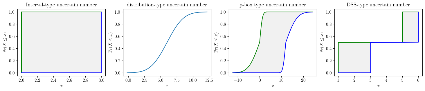
# verbose specification of uncertain numbers
# interval-type uncertain number
a = UN(name='elas_modulus', 
                 symbol='E', 
                 units='Pa', 
                 essence='interval', 
                 intervals=[2,3]
                )

# distribution-type uncertain number
b = UN(
    name='elas_modulus', 
    symbol='E', 
    units='Pa', 
    essence='distribution', 
    distribution_parameters=['gaussian', (6, 2)])

# pbox-type uncertain number
c = UN(
    name='elas_modulus', 
    symbol='E', 
    units='Pa', 
    essence='pbox', 
    distribution_parameters=['gaussian', ([0,12],[1,4])])

# dempster-shafer-type uncertain number
d = UN(
    name='elas_modulus', 
    symbol='E', 
    units='Pa', 
    essence='dempster_shafer', 
    intervals=[[1,5], [3,6]], 
    masses=[0.5, 0.5]
    )

fig, (ax1, ax2, ax3, ax4) = plt.subplots(ncols=4, figsize=(18, 3))
a.plot(ax=ax1, title='Interval-type uncertain number')
b.plot(ax=ax2, title='distribution-type uncertain number')
c.plot(ax=ax3, title='p-box type uncertain number', nuance='curve')
d.plot(ax=ax4, title='DSS-type uncertain number', nuance='curve')
plt.show()

Tip

shortcuts Alternatively, shortcuts existed to instantiate uncertain numbers are also possible when one wants to quickly get on with calculations.

# shortcuts to instantiate uncertain numbers
a = pun.I(2, 3)
b = pun.D('gaussian', (6, 2))
c = pun.normal([0,12], [1,4])
d = pun.DSS([[1,5], [3,6]], [0.5, 0.5])

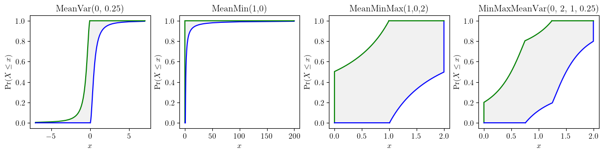
Known constraints

Often there is only partial empirical information (e.g. statistical information) pertaining some variables. A faithful characterisation entails that all of the available statistical information should be utilised but without introducing any extra assumptions beyond what are empirically justified.

fig, axes = plt.subplots(nrows=1, ncols=4, figsize=(12, 3), layout="constrained")
pun.known_constraints(mean=0, var=0.25).plot(title='MeanVar(0, 0.25)', ax=axes[0], nuance='curve')
pun.known_constraints(minimum=0, mean=1).plot(title='MeanMin(1,0)', ax=axes[1], nuance='curve')
pun.known_constraints(minimum=0, mean=1, maximum=2).plot(title='MeanMinMax(1,0,2)', ax=axes[2], nuance='curve')
pun.known_constraints(minimum=0, mean=1, var=0.25, maximum=2).plot(title='MinMaxMeanVar(0, 2, 1, 0.25)', ax=axes[3], nuance='curve')
plt.show()

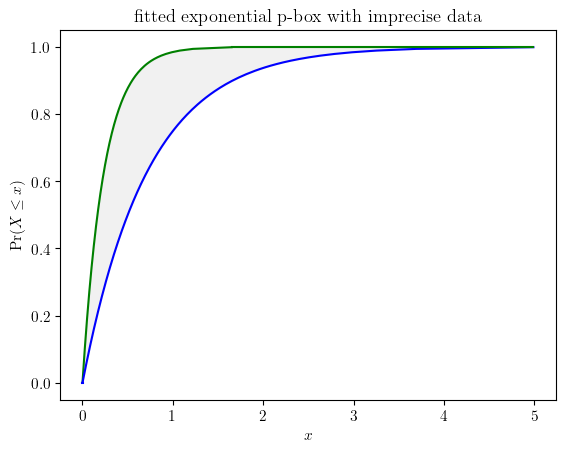
Characterisation from empirical measurements

Empirical data rarely come in perfect forms, especially for in situ measurements. Practical computations frequently deal with poor measurements. Data uncertainty mainly consists of sampling uncertainty and measurement uncertainty. Both parametric and nonparametric estimators are provided to characterise data uncertainties.

from pyuncertainnumber import pba
import scipy.stats as sps

precise_sample = sps.expon(scale=1/0.4).rvs(15)
imprecise_data = pba.I(lo = precise_sample - 1.4, hi=precise_sample + 1.4)

# parametric estimator
fn = pun.fit('mom', family='exponential', data=imprecise_data)
fn.display(title='fitted exponential p-box with imprecise data', nuance='curve')

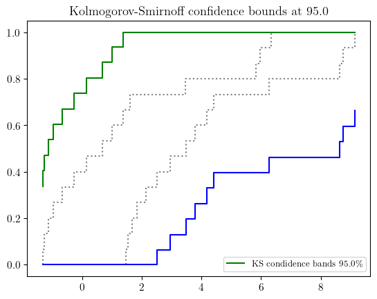
# nonparametric estimator with the KS bounds 
b_l, b_r = pun.KS_bounds(imprecise_data, alpha=0.025, display=True)